Errors in Hypothesis Testing
Hypothesis testing allows researchers to evaluate claims about a population using sample data. We begin with a null hypothesis, $H_0$, which represents the claim being tested, and an alternative hypothesis, $H_a$, which represents a competing claim. Because decisions are based on sample data, errors are possible even when the test is carried out correctly. The two main errors are Type I and Type II errors, and understanding their trade-off is important when designing studies and interpreting results.
Overview of Hypothesis Testing Errors
When performing a hypothesis test, the decision to reject or fail to reject $H_0$ may or may not match the true state of the population:
| Reject $H_0$ | Fail to Reject $H_0$ | |
|---|---|---|
| $H_0$ is True | Type I Error | Correct Decision |
| $H_0$ is False | Correct Decision | Type II Error |
If the null hypothesis is true and we reject it, we make a Type I error. If the null hypothesis is false and we fail to reject it, we make a Type II error.
The Court Trial Analogy
A useful analogy is a court trial. Suppose the null hypothesis represents the claim that a suspect is innocent, while the alternative hypothesis represents the claim that the suspect is guilty.
A conviction corresponds to rejecting the null hypothesis, while an acquittal corresponds to failing to reject it. Convicting an innocent person resembles a Type I error, or false positive. Failing to convict a guilty person resembles a Type II error, or false negative.
The analogy is not exact, but it helps illustrate that different errors can have different consequences and that statistical decisions are made under uncertainty.
Understanding Type I Error (False Positive)
A Type I error occurs when we reject a true null hypothesis. This is commonly called a false positive.
The probability of a Type I error is controlled by the significance level $\alpha$. For example, a test conducted at $\alpha=0.05$ is designed so that, when $H_0$ is true and the assumptions of the test hold, the probability of rejecting $H_0$ is at most about 5%.
Consider a study testing a new drug. If the drug is actually ineffective but the analysis concludes that it is effective, the study has made a Type I error.
The following diagram illustrates the idea. The bell-shaped curve represents the distribution of the test statistic under the null hypothesis, while the critical region marks values that would lead us to reject $H_0$:
         Critical Region (α)
                │
                ▼
         _______________
        /               \
       /                 \
      |   True Null      |   ← Distribution under $H_0$
      |    ($\mu_0$)     |
       \                 /
        \_______________/
Even when $H_0$ is true, random sampling variation can occasionally produce a test statistic that falls in the critical region, causing a false positive.
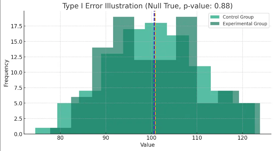
Here, the control and experimental groups have the same population mean, representing a situation in which the null hypothesis is true. Random samples from the two groups can still produce different sample means. If that random difference is large enough to produce a p-value below the chosen significance level, we would reject a true $H_0$ and make a Type I error.
Understanding Type II Error (False Negative)
A Type II error occurs when we fail to reject a false null hypothesis. This is commonly called a false negative.
The probability of a Type II error is denoted by $\beta$. It depends on factors such as sample size, effect size, variability, and the chosen significance level. The probability of correctly detecting an effect when it exists is called the power of the test:
$$ \text{Power}=1-\beta $$
For example, suppose a drug is genuinely effective but the study fails to detect the effect, perhaps because the sample is too small. This would be a Type II error.
The following diagram illustrates the idea. One distribution represents the test statistic under $H_0$, while the other represents its distribution under an alternative hypothesis:
              H0 Distribution              H1 Distribution
             (Centered at $\mu_0$)        (Centered at $\mu_1$)
                    ____                         ____
                   /    \                       /    \
                  /      \                     /      \
                 | $\mu_0$|                   | $\mu_1$|
                  \      /                     \      /
                   \____/                       \____/
                       │
                       ▼  (Critical Threshold)
          Failure to reject $H_0$ can produce a Type II error
If the true effect is not large enough relative to the variability in the data, the observed test statistic may remain outside the rejection region even though $H_0$ is false.
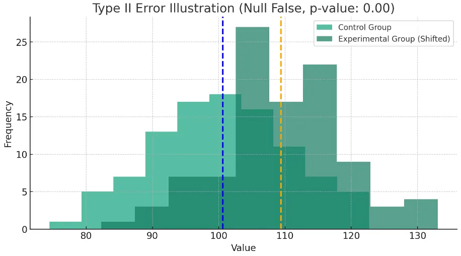
In this plot, the experimental-group mean is shifted to 110 while the control-group mean remains at 100, representing a real difference. If the statistical test fails to detect that difference and we fail to reject $H_0$, a Type II error occurs. The probability of this happening depends on factors such as sample size, effect size, variability, and the chosen significance level.
Balancing Type I and Type II Errors
Type I and Type II errors involve a trade-off. Holding the sample size, effect size, and variability fixed, lowering the significance level $\alpha$ reduces the probability of a Type I error but generally increases $\beta$, the probability of a Type II error.
A more conservative test therefore reduces false positives but may make true effects harder to detect.
The power of the test,
$$ 1-\beta, $$
describes its ability to detect a real effect. Power can often be increased by using a larger sample or reducing measurement variability.
Mathematically:
$$ P(\text{Type I Error}) = \alpha $$
$$ P(\text{Type II Error}) = \beta $$
$$ \text{Power} = 1 - \beta $$
These relationships help researchers balance the risks of false positives and false negatives. The appropriate balance depends on the study and on the consequences of each type of error.
Power Analysis and Sample Size Determination
Power analysis is used to determine the sample size needed to detect an effect of a specified size at a chosen significance level and power. It links four quantities, any three of which determine the fourth:
- Significance level ($\alpha$): the probability of a Type I error.
- Power ($1-\beta$): the probability of correctly rejecting a false $H_0$.
- Effect size ($d$, $r$, $f$, etc.): the magnitude of the difference or relationship the study aims to detect.
- Sample size ($n$): the number of observations.
For a two-sample z-test with equal group sizes, the required sample size per group is approximately:
$$ n \approx \frac{ \left(z_{1-\alpha/2}+z_{1-\beta}\right)^2 \cdot 2\sigma^2 }{ \Delta^2 } $$
where $\Delta=\mu_1-\mu_0$ is the smallest meaningful difference to detect and $\sigma$ is the common standard deviation.
For example, suppose:
- $\alpha=0.05$,
- power $=0.80$, so $\beta=0.20$ and $z_{1-\beta}\approx0.84$,
- $\sigma=10$,
- $\Delta=5$.
Then:
$$ n \approx \frac{ (1.96+0.84)^2\cdot2\cdot100 }{ 25 } $$
$$ n \approx \frac{ 7.84\cdot200 }{ 25 } \approx62.72 $$
so each group would need about 63 observations.
Conducting a power analysis before data collection helps ensure that the study is large enough to detect an effect of practical interest while controlling the risks of Type I and Type II errors.