Linear Regression in Depth
Linear Regression is a fundamental type of supervised learning algorithm in statistics and machine learning. It's utilized for modeling and analyzing the relationship between a dependent variable and one or more independent variables. The goal is to predict continuous output values based on the input variables.
- Purpose: To predict a continuous outcome based on one or more predictor variables.
- Model: The output variable (y) is assumed to be a linear combination of the input variables (x), with coefficients (θ) representing weights.
Mathematical Model
The hypothesis function in linear regression is given by:
$$ h_{\theta}(x) = \theta_0 + \theta_1x $$
where:
- $h_{\theta}(x)$ is the predicted value,
- $\theta_0$ is the y-intercept (bias term),
- $\theta_1$ is the slope (weight for the feature x).
Cost Function (Mean Squared Error)
The cost function in linear regression measures how far off the predictions are from the actual outcomes. It's commonly represented as:
$$ J(\theta_0, \theta_1) = \frac{1}{2m} \sum_{i=1}^{m}(h_{\theta}(x^{(i)}) - y^{(i)})^2 $$
This is the mean squared error (MSE) cost function, where:
- $m$ is the number of training examples,
- $x^{(i)}$ and $y^{(i)}$ are the input and output of the $i^{th}$ training example.
Optimization: Gradient Descent
To find the optimal parameters ($\theta_0$ and $\theta_1$), we use gradient descent to minimize the cost function. The gradient descent algorithm iteratively adjusts the parameters to reduce the cost.
Notation
- $m$: Number of training examples.
- $x$: Input variables/features.
- $y$: Output variable (target variable).
- $(x, y)$: Single training example.
- $(x^{i}, y^{i})$: $i^{th}$ training example.
Training Process
- Input: Training set.
- Algorithm: The learning algorithm processes this data.
- Output: Hypothesis function $h$ which estimates the value of $y$ for a new input $x$.
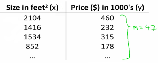
Example: House Price Prediction
Using linear regression, we can predict house prices based on house size.
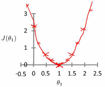
Analyzing the Cost Function
Different values of $\theta_1$ yield different cost (J) values:
- For $\theta_1 = 1$, $J(\theta_1) = 0$ (Ideal scenario).
- For $\theta_1 = 0.5$, $J(\theta_1) = 0.58$ (Higher error).
- For $\theta_1 = 0$, $J(\theta_1) = 2.3$ (Maximum error).
Optimization aims to find the value of $\theta_1$ that minimizes $J(\theta_1)$.
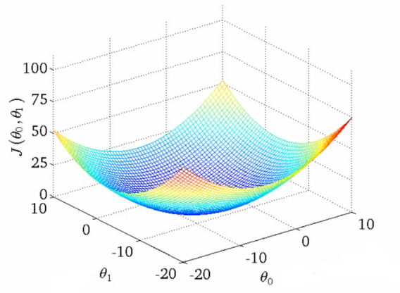
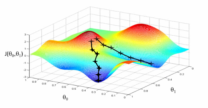
A Deeper Insight into the Cost Function - Simplified Cost Function
In linear regression, the cost function $J(\theta_0, \theta_1)$ is a critical component, involving two parameters: $\theta_0$ and $\theta_1$. Visualization of this function can be achieved through different plots.
3D Surface Plot
The 3D surface plot illustrates the cost function where:
- $X$-axis represents $\theta_1$.
- $Z$-axis represents $\theta_0$.
- $Y$-axis represents $J(\theta_0, \theta_1)$.
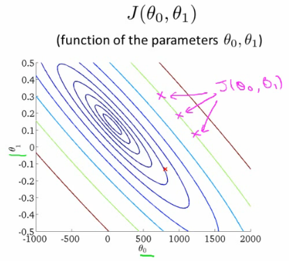
Contour Plots
Contour plots offer a 2D perspective:
- Each color or level represents the same value of $J(\theta_0, \theta_1)$.
- The center of concentric circles indicates the minimum of the cost function.
Gradient Descent Algorithm
The gradient descent algorithm iteratively adjusts $\theta_0$ and $\theta_1$ to minimize the cost function. The algorithm proceeds as follows:
θ = [0, 0]
while not converged:
    for j in [0, 1]:
θ_j := θ_j - α ∂/∂θ_j J(θ_0, θ_1)- Begin with initial guesses (e.g., [0,0]).
- Continuously adjust $\theta_0$ and $\theta_1$ to reduce $J(\theta_0, \theta_1)$.
- Proceed until a local minimum is reached.
Here is a complete Python code that generates mock data and implements the gradient descent algorithm to fit a linear regression model. The code also includes plotting the cost function and the path taken by the gradient descent algorithm.
import numpy as np
import matplotlib.pyplot as plt

# Generate mock data
np.random.seed(42)
X = 2 * np.random.rand(100, 1)
y = 4 + 3 * X + np.random.randn(100, 1)

# Feature normalization
X_mean = np.mean(X)
X_std = np.std(X)
X_norm = (X - X_mean) / X_std

# Add bias term (X0 = 1)
X_b = np.c_[np.ones((100, 1)), X_norm]

# Initialize parameters
theta = np.random.randn(2, 1) * 0.01
alpha = 0.1
n_iterations = 1000
m = len(X_b)
tolerance = 1e-7

# Cost function
def compute_cost(theta, X_b, y):
    return (1 / (2 * m)) * np.sum((X_b.dot(theta) - y) ** 2)

# Gradient Descent
cost_history = []
theta_history = [theta]

for iteration in range(n_iterations):
    gradients = (1 / m) * X_b.T.dot(X_b.dot(theta) - y)
    theta = theta - alpha * gradients
    cost = compute_cost(theta, X_b, y)
    cost_history.append(cost)
    theta_history.append(theta.copy())
    if len(cost_history) > 1 and np.abs(cost_history[-1] - cost_history[-2]) < tolerance:
        break

# Prepare data for contour plot
theta_0_vals = np.linspace(-10, 10, 100)
theta_1_vals = np.linspace(-4, 4, 100)
cost_vals = np.zeros((len(theta_0_vals), len(theta_1_vals)))

for i in range(len(theta_0_vals)):
    for j in range(len(theta_1_vals)):
        theta_ij = np.array([[theta_0_vals[i]], [theta_1_vals[j]]])
        cost_vals[i, j] = compute_cost(theta_ij, X_b, y)

# Plotting
fig, ax = plt.subplots(figsize=(10, 6))

# Contour plot
theta_0_vals, theta_1_vals = np.meshgrid(theta_0_vals, theta_1_vals)
CS = ax.contour(theta_0_vals, theta_1_vals, cost_vals, levels=np.logspace(-2, 3, 20), cmap='viridis')
ax.clabel(CS, inline=1, fontsize=10)

# Plot the path of the gradient descent
theta_history = np.array(theta_history)
ax.plot(theta_history[:, 0], theta_history[:, 1], 'r-o', label='Gradient Descent Path')

# Annotate the start and end points
ax.annotate('Start', xy=(theta_history[0, 0], theta_history[0, 1]), xytext=(-9, 3),
            arrowprops=dict(facecolor='black', shrink=0.05), fontsize=12, color='black')
ax.annotate('End', xy=(theta_history[-1, 0], theta_history[-1, 1]), xytext=(theta_history[-1, 0] + 1, theta_history[-1, 1]),
            arrowprops=dict(facecolor='black', shrink=0.05), fontsize=12, color='black')

ax.set_xlabel(r'$\theta_0$', fontsize=14)
ax.set_ylabel(r'$\theta_1$', fontsize=14)
ax.set_title('Gradient Descent Path')
ax.legend()

plt.show()

# Plot cost function
plt.figure(figsize=(8, 4))
plt.plot(cost_history, 'b-', label='Cost Function')
plt.xlabel('Iterations')
plt.ylabel('Cost')
plt.title('Cost Function Over Iterations')
plt.legend()
plt.show()- The code begins by importing the necessary libraries: numpy for numerical operations and matplotlib.pyplot for plotting.
- Random data generation is performed using a fixed seed for reproducibility, producing 100 data points for the feature variable X and the target variable y, which follows a linear relationship with added Gaussian noise.
- To normalize the features, the code calculates the mean and standard deviation of X, then scales the feature by subtracting the mean and dividing by the standard deviation.
- A bias term (a column of ones) is added to the feature matrix X to account for the intercept in the linear regression model.
- The initial parameters for the linear regression model, referred to as theta, are initialized with small random values. The learning rate (alpha) is set to 0.1, and the number of iterations for gradient descent is set to 1000. The number of training examples (m) is determined from the dataset.
- The cost function, which measures the mean squared error between the predicted and actual values, is defined to evaluate the performance of the model.
- Gradient descent is implemented to optimize the parameters theta. In each iteration, the gradients of the cost function with respect to the parameters are computed, and the parameters are updated in the direction that minimizes the cost.
- A history of the cost function values and parameter updates is maintained during the gradient descent iterations. The algorithm terminates early if the change in the cost function value between consecutive iterations falls below a specified tolerance level.
- For visualization purposes, a range of theta values is prepared, and the cost function is evaluated across this range to create a contour plot, showing the cost landscape.
- The code generates a contour plot that illustrates the cost function values for different theta values. It also plots the path taken by gradient descent, highlighting the start and end points of the optimization process.
- Additionally, the code plots the cost function values over the iterations to show how the cost decreases as gradient descent progresses.
Below is the gradient descent path:
And here is the cost function over iterations:
Key Elements of Gradient Descent
- Learning Rate ($\alpha$): Determines the step size during each iteration.
- Partial Derivative: Indicates the direction to move in the parameter space.
- A negative derivative suggests a decrease in $\theta_1$ to move towards a minimum.
- Conversely, a positive derivative suggests an increase in $\theta_1$.
Partial Derivative vs. Derivative
- Partial Derivative: Applied when focusing on a single variable among several.
- Derivative: Utilized when considering all variables.
At a Local Minimum
At this point, the derivative equals zero, implying no further changes in $\theta_1$:
$$ \alpha \times 0 = 0 \Rightarrow \theta_1 = \theta_1 - 0 $$

Through gradient descent, the optimal $\theta_0$ and $\theta_1$ values are identified, minimizing the cost function and enhancing the linear regression model's performance.
Linear Regression with Gradient Descent
In linear regression, gradient descent is applied to minimize the squared error cost function $J(\theta_0, \theta_1)$. The process involves calculating the partial derivatives of the cost function with respect to each parameter $\theta_0$ and $\theta_1$.
Partial Derivatives of the Cost Function
The gradient of the cost function is computed as follows:
- For the squared error cost function:
$$\frac{\partial}{\partial \theta_j} J(\theta_0, \theta_1) = \frac{\partial}{\partial \theta_j} \frac{1}{2m} \sum_{i=1}^{m} (h_{\theta}(x^{(i)}) - y^{(i)})^2$$
$$= \frac{\partial}{\partial \theta_j} \frac{1}{2m} \sum_{i=1}^{m} (\theta_0 + \theta_1x^{(i)} - y^{(i)})^2$$
The partial derivatives for each $\theta_j$ are:
- For $j=0$:
$$\frac{\partial}{\partial \theta_0} J(\theta_0, \theta_1)=\frac{\partial}{\partial \theta_0} \frac{1}{m} \sum_{i=1}^{m} (h_{\theta}(x^{(i)}) - y^{(i)})$$
- For $j=1$:
$$\frac{\partial}{\partial \theta_1} J(\theta_0, \theta_1)=\frac{\partial}{\partial \theta_1} \frac{1}{m} \sum_{i=1}^{m} (h_{\theta}(x^{(i)}) - y^{(i)})x^{(i)}$$
Normal Equations Method
For solving the minimization problem $\min J(\theta_0, \theta_1)$, the normal equations method offers an alternative to gradient descent. This numerical method provides an exact solution, avoiding the iterative approach of gradient descent. It can be faster for certain problems but is more complex and will be covered in detail later.
Below is the Python code to generate mock data and solve the minimization problem (\min J(\theta_0, \theta_1)) using the normal equations method.
import numpy as np
import matplotlib.pyplot as plt

# Generate mock data
np.random.seed(42)
X = 2 * np.random.rand(100, 1)
y = 4 + 3 * X + np.random.randn(100, 1)

# Add bias term (X0 = 1)
X_b = np.c_[np.ones((100, 1)), X]

# Normal Equations method
theta_best = np.linalg.inv(X_b.T.dot(X_b)).dot(X_b.T).dot(y)

# Display the results
print(f"Theta obtained by the Normal Equations method: {theta_best.ravel()}")

# Plotting the results
plt.figure(figsize=(10, 6))
plt.plot(X, y, 'b.', label='Data Points')
plt.plot(X, X_b.dot(theta_best), 'r-', label='Prediction', linewidth=2)
plt.xlabel('X')
plt.ylabel('y')
plt.title('Linear Regression using Normal Equations')
plt.legend()
plt.show()- The data generation begins with setting a random seed using
np.random.seed(42)to ensure reproducibility of the results. - The feature variable $X$ is generated as 100 random values between 0 and 2, using the $np.random.rand$ function and scaling by 2.
- The target variable $y$ is generated using a linear relationship with the feature variable $X$, specifically $y = 4 + 3X$, and includes added Gaussian noise using $np.random.randn$ to simulate real-world data variability.
- A bias term, represented as a column of ones, is added to the feature matrix $X$ to account for the intercept term in the linear regression model. This is achieved by concatenating the bias term with $X$ to form $X_b$.
- The normal equations method is used to solve for the optimal parameters $\theta$. This method calculates the parameters directly by solving the equation $(X_b^T X_b)^{-1} X_b^T y$.
- This approach avoids the iterative process used in gradient descent and provides an exact solution for the linear regression parameters.
- The computed parameters $\theta_{\text{best}}$ are then printed to the console, showing the values obtained by the normal equations method.
- To visualize the results, a plot is generated with matplotlib. The data points are plotted as blue dots, and the fitted linear regression line is plotted as a red line.
Extension of the Current Model
The linear regression model can be extended to include multiple features. For example, in a housing model, features could include size, age, number of bedrooms, and number of floors. However, a challenge arises when dealing with more than three dimensions, as visualization becomes difficult. To effectively manage multiple features, linear algebra concepts like matrices and vectors are employed, facilitating calculations and interpretations in higher-dimensional spaces.
Reference
These notes are based on the free video lectures offered by Stanford University, led by Professor Andrew Ng. These lectures are part of the renowned Machine Learning course available on Coursera. For more information and to access the full course, visit the Coursera course page.