Linear Algebra Review

Linear Algebra forms the backbone of many machine learning algorithms, including linear regression. Understanding matrices and vectors is fundamental in this context.

Matrices Overview

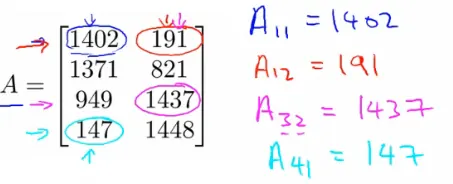
• Definition: Matrices are rectangular arrays of numbers enclosed in square brackets. They are the cornerstone of organizing and manipulating large sets of data.
• Notation: Typically denoted by uppercase letters (e.g., A, B, X, Y).
• Dimensions: Expressed as [Rows x Columns]. The entry in the $i^{th}$ row and $j^{th}$ column of a matrix A is denoted as $A_{(i,j)}$.

Vectors Overview

• Definition: A vector is a special type of matrix with only one column (n x 1 matrix).
• Notation: Usually represented by lowercase letters. The $i^{th}$ element of vector $v$ is denoted as $v_i$.
• Usage: Vectors are used to represent data points or features in machine learning.

Vector Representation

A vector can be represented as:

$$ y = \begin{bmatrix} x_{1} \\ x_{2} \\ \vdots \\ x_{m} \end{bmatrix} $$

where $x_{1}, x_{2}, ..., x_{m}$ are the elements of the vector.

Matrix Manipulation

Understanding matrix manipulation is essential in linear algebra and machine learning for organizing and processing data. Here are some fundamental operations:

Matrix Addition

Element-wise addition of two matrices of the same dimension.

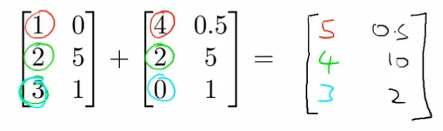
Important: The matrices must have the same number of rows and columns.

Multiplication by Scalar

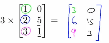
Multiplying every element of a matrix by a scalar value.

Multiplication by Vector

Multiplying a matrix with a vector.

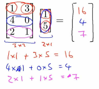
Important: The number of columns in the matrix must equal the number of elements in the vector.

Multiplication by Another Matrix

Combining two matrices.

Procedure:

• Multiply matrix A with each column vector of matrix B.
• This results in a new matrix where each column is the result of multiplying A with a column of B.

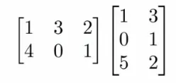
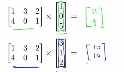
Important: The number of columns in the first matrix must match the number of rows in the second matrix.

Matrix Multiplication Properties

Matrix multiplication, a crucial operation in linear algebra, has specific properties that distinguish it from scalar multiplication.

Lack of Commutativity

I. For real numbers, multiplication is commutative.

$$3 \cdot 5 == 5 \cdot 3$$

II. The commutative property does not hold for matrix multiplication.

$$A \times B \neq B \times A$$

Associativity

I. Associative property holds for multiplication of real numbers.

$$3 \cdot (5 \cdot 2) == (3 \cdot 5) \cdot 2$$

II. Matrix multiplication is associative.

$$A \times (B \times C) == (A \times B) \times C$$

Identity Matrix

I. In scalar multiplication, 1 is the identity element.

$$z \cdot 1 = z$$

II. For matrices, the identity matrix $I$ serves as the identity element.

$$ I = \begin{bmatrix} 1 & 0 & 0 \\ 0 & 1 & 0 \\ 0 & 0 & 1 \end{bmatrix} $$

When multiplied by any compatible matrix $A$, it results in $A$ itself.

$$A \times I = A$$

Matrix Inverse

I. For non-zero real numbers, the multiplicative inverse holds.

$$x \cdot \frac{1}{x} = 1$$

II. Only square matrices can have an inverse. Not every square matrix has an inverse, analogous to how 0 has no multiplicative inverse in real numbers. Finding matrix inverses involves specific numerical methods.

Matrix Transpose

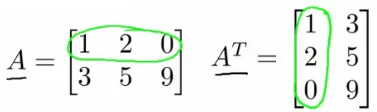
The transpose of a matrix $A$ of size $m \times n$ is another matrix $B$ of size $n \times m$, where the elements are flipped over its diagonal.

$B_{(j,i)} = A_{(i,j)}$.

Application in Machine Learning

• Data Representation: Matrices and vectors are used to represent datasets, where each row can be a data point and columns are the features.
• Model Representation: In linear regression, the hypothesis can be represented as a matrix-vector product, simplifying the computation and representation of multiple features.
• Efficiency: Linear algebra operations, especially when implemented in optimized libraries, provide efficient computation for large datasets.

Example: House Prices

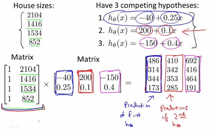
Suppose there are multiple hypotheses to predict house prices based on different factors. With a dataset of house sizes, these hypotheses can be applied simultaneously using matrix operations.

For four houses and three different hypotheses:

• Convert the data into a $4 \times 2$ matrix by adding an extra column of ones (to account for the bias term in linear regression).
• Multiply this matrix with a matrix containing the parameters of the hypotheses.

This approach demonstrates how matrix multiplication can streamline the application of multiple hypotheses to a dataset, enhancing efficiency and scalability.

Reference

These notes are based on the free video lectures offered by Stanford University, led by Professor Andrew Ng. These lectures are part of the renowned Machine Learning course available on Coursera. For more information and to access the full course, visit the Coursera course page.