Linear Regression with Multiple Variables

Last modified: July 10, 2024

This article is written in: 🇺🇸

Linear Regression with Multiple Variables

Multiple linear regression extends the concept of simple linear regression to multiple independent variables. This technique models a dependent variable as a linear combination of several independent variables.

Variables: The model uses several variables (or features), such as house size, number of bedrooms, floors, and age.
$n$: Number of features (e.g., 4 in our example).
$m$: Number of examples (rows in data).
$x^i$: Feature vector of the $i^{th}$ training example.
$x_j^i$: Value of the $j^{th}$ feature in the $i^{th}$ training set.

Hypothesis Function

The hypothesis in multiple linear regression combines all the features:

$$ h_{\theta}(x) = \theta_0 + \theta_1x_1 + \theta_2x_2 + \theta_3x_3 + \theta_4x_4 $$

For simplification, introduce $x_0 = 1$ (bias term), making the feature vector $n + 1$-dimensional.

$$ h_{\theta}(x) = \theta^T X $$

Cost Function

The cost function measures the discrepancy between the model's predictions and actual values. It is defined as:

$$ J(\theta_0, \theta_1, ..., \theta_n) = \frac{1}{2m} \sum_{i=1}^{m}(h_{\theta}(x^{(i)}) - y^{(i)})^2 $$

Gradient Descent for Multiple Variables

Gradient descent is employed to find the optimal parameters that minimize the cost function.

θ = [0] * n
while not converged:
  for j in [0, ..., n]:
      θ_j := θ_j - α ∂/∂θ_j J(θ_0, ..., θ_n)

Simultaneous Update: Adjust each $\theta_j$ (from 0 to nn) simultaneously.
Learning Rate ($\alpha$): Determines the step size in each iteration.
Partial Derivative: Represents the direction and rate of change of the cost function with respect to each $\theta_j$.

Here is a Python code that demonstrates the gradient descent algorithm for multiple variables with mock data:

import numpy as np

# Mock data
# Features (x0, x1, x2)
X = np.array([
    [1, 2, 3],
    [1, 3, 4],
    [1, 4, 5],
    [1, 5, 6]
])

# Target values
y = np.array([7, 10, 13, 16])

# Parameters
alpha = 0.01  # Learning rate
num_iterations = 1000  # Number of iterations for gradient descent

# Initialize theta (parameters) to zeros
theta = np.zeros(X.shape[1])

# Cost function
def compute_cost(X, y, theta):
    m = len(y)
    predictions = X.dot(theta)
    cost = (1 / (2 * m)) * np.sum((predictions - y) ** 2)
    return cost

# Gradient descent algorithm
def gradient_descent(X, y, theta, alpha, num_iterations):
    m = len(y)
    cost_history = np.zeros(num_iterations)
    
    for iteration in range(num_iterations):
        # Compute the prediction error
        error = X.dot(theta) - y
        
        # Update theta values simultaneously
        for j in range(len(theta)):
            partial_derivative = (1 / m) * np.sum(error * X[:, j])
            theta[j] = theta[j] - alpha * partial_derivative
        
        # Save the cost for the current iteration
        cost_history[iteration] = compute_cost(X, y, theta)
    
    return theta, cost_history

# Run gradient descent
theta, cost_history = gradient_descent(X, y, theta, alpha, num_iterations)

print("Optimized theta:", theta)
print("Final cost:", cost_history[-1])

# Plotting the cost function history
import matplotlib.pyplot as plt

plt.plot(range(num_iterations), cost_history, 'b')
plt.xlabel('Number of iterations')
plt.ylabel('Cost J')
plt.title('Cost function history')
plt.show()

In the context of multiple variables, gradient descent adjusts each parameter theta simultaneously.
The cost function typically measures the difference between predicted and actual values.
A common cost function used in linear regression is the mean squared error.
The learning rate, represented by alpha, determines the step size in each iteration of gradient descent.
Choosing an appropriate learning rate is crucial, as too high a value can cause divergence, while too low a value can slow convergence.
Gradient descent involves computing the partial derivative of the cost function with respect to each parameter theta.
The partial derivative indicates the direction and rate of change of the cost function concerning a specific parameter.
In each iteration, the parameters are updated by subtracting the product of the learning rate and the partial derivative.
The process continues until the parameters converge, meaning changes in the cost function are minimal.
To visualize the convergence, the cost function value is often plotted over iterations.
Mock data can be used to illustrate the gradient descent process, involving features matrix X and target values vector y.
Initialization of parameters to zeros is a common starting point in gradient descent.
The prediction error is calculated as the difference between the predicted values and the actual target values.
Updating theta values involves iterating through each parameter and adjusting it based on the computed partial derivatives.
Tracking the cost function value at each iteration helps in understanding the convergence behavior.
The optimized theta values are obtained after the specified number of iterations or when convergence criteria are met.

Figure_1

Feature Scaling

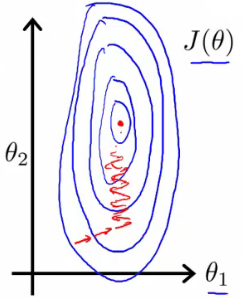
When features have different scales, gradient descent may converge slowly.

Example: If $x_1$ = size (0 - 2000 feet) and $x_2$ = number of bedrooms (1-5), the cost function contours become skewed, leading to a longer path to convergence.
Solution: Scale the features to have comparable ranges.

feature_scaling

Here is the Python code that focuses on feature scaling using mock data:

import numpy as np

# Mock data
# Features (x0, x1, x2)
X = np.array([
    [1, 2000, 3],
    [1, 1600, 4],
    [1, 2400, 2],
    [1, 3000, 5]
])

# Function to perform feature scaling
def feature_scaling(X):
    # Exclude the first column (intercept term)
    X_scaled = X.copy()
    for i in range(1, X.shape[1]):
        mean = np.mean(X[:, i])
        std = np.std(X[:, i])
        X_scaled[:, i] = (X[:, i] - mean) / std
    return X_scaled

# Apply feature scaling
X_scaled = feature_scaling(X)

print("Original Features:\n", X)
print("Scaled Features:\n", X_scaled)

In the context of implementing feature scaling in Python, one would first compute the mean and standard deviation of each feature.
The next step involves adjusting each feature value by subtracting the mean and dividing by the standard deviation.
This transformation ensures that each feature contributes equally to the cost function, facilitating faster and more stable convergence of gradient descent.
The feature scaling process is crucial for algorithms that rely on distance measurements, such as gradient descent, as it helps in achieving better performance and accuracy.
By scaling features appropriately, one can prevent the gradient descent algorithm from being dominated by features with larger scales, ensuring a more balanced optimization process.

Mean Normalization

Adjust each feature $x_i$ by subtracting the mean and dividing by the range (max - min).

mean_normalization

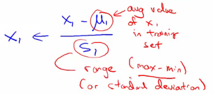
Transforms the features to have approximately zero mean, aiding in faster convergence.

Below is the Python code that demonstrates mean normalization using mock data:

import numpy as np

# Mock data
# Features (x0, x1, x2)
X = np.array([
    [1, 2000, 3],
    [1, 1600, 4],
    [1, 2400, 2],
    [1, 3000, 5]
])

# Function to perform mean normalization
def mean_normalization(X):
    # Exclude the first column (intercept term)
    X_normalized = X.copy()
    for i in range(1, X.shape[1]):
        mean = np.mean(X[:, i])
        min_val = np.min(X[:, i])
        max_val = np.max(X[:, i])
        X_normalized[:, i] = (X[:, i] - mean) / (max_val - min_val)
    return X_normalized

# Apply mean normalization
X_normalized = mean_normalization(X)

print("Original Features:\n", X)
print("Mean Normalized Features:\n", X_normalized)

The purpose of mean normalization is to transform the features so that they have approximately zero mean, which aids in faster convergence of optimization algorithms like gradient descent.
When features have different scales, optimization algorithms may converge slowly or get stuck in local minima. Mean normalization helps to bring all features to a similar scale.
In the process of mean normalization, for each feature, the mean value is first calculated.
Next, the range of the feature is determined by subtracting the minimum value from the maximum value.
Each feature value is then adjusted by subtracting the mean and dividing by the range. This results in features with values centered around zero.
Mean normalization is particularly useful for algorithms that are sensitive to the scale of input features, such as gradient descent.
By ensuring that features have similar scales, mean normalization prevents features with larger scales from dominating the learning process.
The transformed features, having approximately zero mean, contribute to a more balanced and efficient optimization process.
In Python we are iterating over each feature, computing the mean, minimum, and maximum values, and applying the normalization formula.
This preprocessing step is crucial for improving the performance of machine learning models, especially those relying on distance measurements or gradient-based optimization.

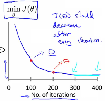
Learning Rate $\alpha$

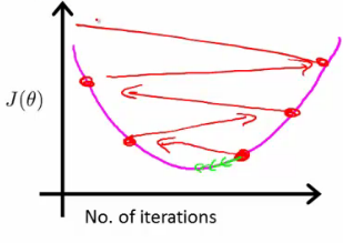
Monitoring: Plot $\min J(\theta)$ against the number of iterations to observe how $J(\theta)$ decreases.
Signs of Proper Functioning: $J(\theta)$ should decrease with every iteration.
Iterative Adjustment: Avoid hard-coding iteration thresholds. Instead, use results to adjust future runs.

min_cost_function

Automatic Convergence Tests

Goal: Determine if $J(\theta)$ changes by a small enough threshold, indicating convergence.
Challenge: Choosing an appropriate threshold can be difficult.
Indicator of Incorrect $\alpha$: If $J(\theta)$ increases, it suggests the need for a smaller learning rate.

alpha_big

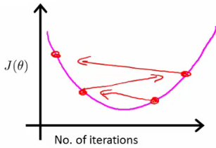
Adjusting $\alpha$: If the learning rate is too high, you might overshoot the minimum. Conversely, if $\alpha$ is too small, convergence becomes inefficiently slow.

alpha_small

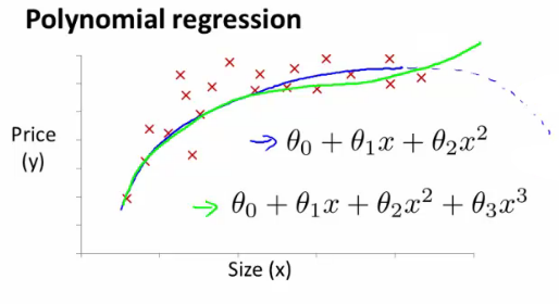
Features and Polynomial Regression

Polynomial Regression: An advanced form of linear regression where the relationship between the independent variable $x$ and the dependent variable $y$ is modeled as an $n^{th}$ degree polynomial.
Application: Can fit data better than simple linear regression by capturing non-linear relationships.
Consideration: Balancing between overfitting (too complex model) and underfitting (too simple model).

polynomial_regression

Normal Equation

Normal Equation: Provides an analytical solution to the linear regression problem.
Alternative to Gradient Descent: Unlike the iterative nature of gradient descent, the normal equation solves for $\theta$ directly.

Procedure

$\theta$ is an $n+1$ dimensional vector.
The cost function $J(\theta)$ takes $\theta$ as an argument.
Minimize $J(\theta)$ by setting its partial derivatives with respect to $\theta_j$ to zero and solving for each $\theta_j$.

Example

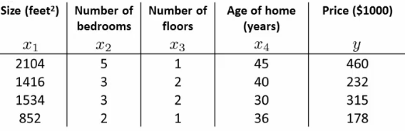
Given $m=4$ training examples and $n=4$ features.
Add an extra column $x_0$ (bias term) to form an $[m \times n+1]$ matrix (design matrix X).
Construct a $[m \times 1]$ column vector $y$.
Calculate $\theta$ using:

$$ \theta = (X^TX)^{-1}X^Ty $$

normal_eq_table normal_eq_matrix

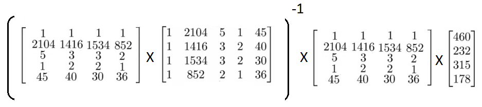
The computed $\theta$ values minimize the cost function for the given training data.

Here is the Python code that uses the provided data to solve for ( \theta ) using the normal equation, and then plots the solution:

import numpy as np
import matplotlib.pyplot as plt

# Given data
# Features (x0, x1, x2, x3, x4)
X = np.array([
    [1, 2104, 5, 1, 45],
    [1, 1416, 3, 2, 40],
    [1, 1534, 3, 2, 30],
    [1, 852, 2, 1, 36]
])

# Target values
y = np.array([460, 232, 315, 178])

# Normal equation: theta = (X^T * X)^-1 * X^T * y
def normal_equation(X, y):
    X_transpose = X.T
    theta = np.linalg.inv(X_transpose.dot(X)).dot(X_transpose).dot(y)
    return theta

# Calculate theta using the normal equation for multivariable regression
theta = normal_equation(X, y)
print("Calculated theta values for multivariable regression:", theta)

# Using the first feature (size) for plotting the regression line
sizes = X[:, 1]
predicted_prices = X.dot(theta)

# Plotting the regression line for multivariable regression
plt.scatter(sizes, y, color='red', label='Actual Prices')
plt.plot(sizes, predicted_prices, color='blue', label='Predicted Prices', linestyle='--')
plt.xlabel('Size (square feet)')
plt.ylabel('Price ($1000)')
plt.title('House Prices vs. Size (Multivariable Regression)')
plt.legend()
plt.show()

# Simple Linear Regression with size as the only feature
X_simple = X[:, [0, 1]]  # Only intercept term and size feature
theta_simple = normal_equation(X_simple, y)

# Predicting using the model with only size
predicted_prices_simple = X_simple.dot(theta_simple)

# Sorting the data by size for a proper line plot
sorted_indices = X[:, 1].argsort()
sizes_sorted = sizes[sorted_indices]
y_sorted = y[sorted_indices]
predicted_prices_sorted = predicted_prices_simple[sorted_indices]

# Plotting the regression line with size as the only feature
plt.scatter(sizes, y, color='red', label='Actual Prices')
plt.plot(sizes_sorted, predicted_prices_sorted, color='blue', label='Predicted Prices', linestyle='--')
plt.xlabel('Size (square feet)')
plt.ylabel('Price ($1000)')
plt.title('House Prices vs. Size (Simple Linear Regression)')
plt.legend()
plt.show()

print("Calculated theta values for simple linear regression:", theta_simple)

To implement the normal equation, the transpose of the design matrix ( X ) is first computed. This step involves swapping the rows and columns of ( X ).
Next, the product of the transpose of ( X ) and ( X ) is calculated, resulting in a square matrix.
The inverse of this square matrix is then found. This step can be computationally expensive for large matrices but is feasible for smaller datasets.
The result of the inversion is then multiplied by the transpose of ( X ) and the target vector ( y ) to obtain the parameter vector ( \theta ).
Using the calculated ( \theta ) values, predictions can be made by multiplying the design matrix ( X ) by ( \theta ).
To validate the model, the predicted values are compared with the actual target values. Plotting these values can help visualize the model's performance.
In the given example, the design matrix ( X ) includes an intercept term and features such as size, number of bedrooms, number of floors, and age of the house. The target vector ( y ) represents house prices.
The normal equation provides a straightforward solution for linear regression problems, especially when the number of features is relatively small. It eliminates the need for tuning hyperparameters like the learning rate and avoids the iterative nature of gradient descent.
However, for datasets with a large number of features, the normal equation can become computationally impractical due to the matrix inversion step.

output(5)

Gradient Descent vs Normal Equation

Comparing these two methods helps understand their practical applications:

Aspect	Gradient Descent	Normal Equation
Learning Rate	Requires selecting a learning rate	No learning rate needed
Iterations	Numerous iterations needed	Direct computation without iterations
Efficiency	Works well for large $n$ (even millions)	Becomes slow for large $n$
Use Case	Preferred for very large feature sets	Ideal for smaller feature sets

Understanding when to use polynomial regression, and choosing between gradient descent and the normal equation, is crucial in developing efficient and effective linear regression models.

Reference

These notes are based on the free video lectures offered by Stanford University, led by Professor Andrew Ng. These lectures are part of the renowned Machine Learning course available on Coursera. For more information and to access the full course, visit the Coursera course page.