Advice for Applying Machine Learning Techniques and Debugging Learning Algorithms

Last modified: June 23, 2024

This article is written in: 🇺🇸

Advice for Applying Machine Learning Techniques and Debugging Learning Algorithms

Troubleshooting High Error Rates

When facing high error rates with a machine learning model, especially when tested on new data, various strategies can be employed to diagnose and address the problem.

Steps for Improvement

Add More Training Data: Sometimes, the model has not seen enough examples to generalize well.
Add or Remove Features: The model might be missing key features that are important for predictions or might be overwhelmed by irrelevant or noisy features.
Adjust Regularization Parameter ($\lambda$): If the model is overfitting, increasing the regularization parameter can help. If underfitting, decreasing it might be beneficial.
Data Splitting: Divide your dataset into a training set and a test set to assess model performance on unseen data.
Model Selection with Validation Set: Create a training, validation, and test set to tune and select the best model.
Polynomial Degree Analysis: Plot errors for training and validation sets against polynomial degrees to diagnose high bias (underfitting) or high variance (overfitting).
Advanced Optimization Algorithms: Employ sophisticated optimization techniques to minimize the cost function more effectively.

Debugging a Learning Algorithm

Consider a scenario where you have used regularized linear regression to predict home prices, but the model yields high errors on new data.

Cost Function

Use the cost function for the regularized linear regression:

$$ J(\theta) = \frac{1}{2m} \left[ \sum_{i=1}^{m}(h_{\theta}(x^{(i)} - y^{(i)})^2 + \lambda \sum_{j=1}^{m} \theta_j^2 \right] $$

Next Steps for Improvement

Obtain More Training Data: Helps the algorithm to better generalize.
Reduce Feature Set: Try using fewer features to avoid overfitting.
Incorporate More Features: Add new features that might be relevant.
Add Polynomial Features: Enables the model to capture more complex relationships.
Modify $\lambda$: Adjust the regularization parameter to find the right balance between bias and variance.

Evaluating the Hypothesis

Evaluating the model’s performance involves splitting the data and computing errors:

Data Split

Training Set: Used to learn the parameters, $\theta$.
Test Set: Used to compute the test error.

Here is a simple implementation to split the data into a training set and a test set, train a logistic regression model on the training set, and evaluate it on the test set:

import numpy as np
from sklearn.linear_model import LogisticRegression
from sklearn.metrics import accuracy_score
from sklearn.model_selection import train_test_split

# Mock data
X = np.array([[0.5, 1.5],
              [1.5, 0.5],
              [3, 3.5],
              [2, 2.5],
              [1, 1],
              [3.5, 4],
              [2.5, 3],
              [1, 0.5]])
y = np.array([0, 0, 1, 1, 2, 2, 1, 0])  # 0: Triangle, 1: Cross, 2: Square

# Binary classification for simplicity (convert multi-class to binary problem)
y_binary = (y == 1).astype(int)

# Split data into training and test sets
X_train, X_test, y_train, y_test = train_test_split(X, y_binary, test_size=0.3, random_state=42)

# Initialize the logistic regression model
model = LogisticRegression()

# Train the model on the training set
model.fit(X_train, y_train)

# Make predictions on the test set
y_test_pred = model.predict(X_test)

# Evaluate the model
test_accuracy = accuracy_score(y_test, y_test_pred)

print("Test Accuracy:", test_accuracy)
print("Test Predictions:", y_test_pred)
print("Actual Labels:", y_test)

Test Error Calculation

Compute the test error using the learned parameters:

$$J_{test}(\theta) = \frac{1}{2m_{test}} \sum_{i=1}^{m_{test}}(h_{\theta}(x^{(i)}{test} - y^{(i)}{test})^2$$

This step helps to evaluate how well the model generalizes to new, unseen data.

To compute the test error for a logistic regression model using the mean squared error (MSE) formula provided, you can follow these steps:

import numpy as np
from sklearn.linear_model import LogisticRegression
from sklearn.model_selection import train_test_split

# Sigmoid function
def sigmoid(z):
    return 1 / (1 + np.exp(-z))

# Hypothesis function
def hypothesis(theta, X):
    return sigmoid(np.dot(X, theta))

# Test error function
def compute_test_error(theta, X_test, y_test):
    m_test = len(y_test)
    h = hypothesis(theta, X_test)
    error = (1 / (2 * m_test)) * np.sum((h - y_test) ** 2)
    return error

# Example usage
if __name__ == "__main__":
    # Sample data
    X = np.array([[0.5, 1.5],
                  [1.5, 0.5],
                  [3, 3.5],
                  [2, 2.5],
                  [1, 1],
                  [3.5, 4],
                  [2.5, 3],
                  [1, 0.5]])
    y = np.array([0, 0, 1, 1, 2, 2, 1, 0])  # 0: Triangle, 1: Cross, 2: Square

    # Binary classification for simplicity (convert multi-class to binary problem)
    y_binary = (y == 1).astype(int)

    # Split data into training and test sets
    X_train, X_test, y_train, y_test = train_test_split(X, y_binary, test_size=0.3, random_state=42)

    # Initialize the logistic regression model
    model = LogisticRegression()

    # Train the model on the training set
    model.fit(X_train, y_train)

    # Get the learned parameters
    theta = np.hstack([model.intercept_, model.coef_[0]])

    # Add intercept term to test set
    X_test = np.hstack([np.ones((X_test.shape[0], 1)), X_test])

    # Compute the test error
    test_error = compute_test_error(theta, X_test, y_test)

    print("Test Error:", test_error)

Model Selection Process

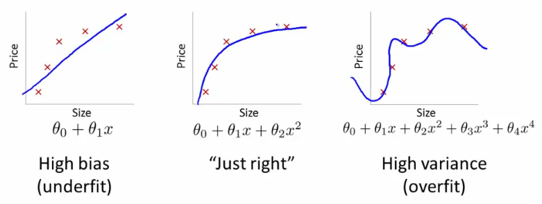
When applying machine learning algorithms, selecting the right model and parameters is crucial. This includes choosing the regularization parameter or the polynomial degree for regression models. The challenge is to balance between underfitting (high bias) and overfitting (high variance).

Determine Polynomial Degree (d): You may want to choose between different degrees of polynomial models, ranging from linear ($d=1$) to higher-degree polynomials.

For example, models can range from $h_{\theta}(x) = \theta_0 + \theta_1x$ to $h_{\theta}(x) = \theta_0 + ... + \theta_{10}x^{10}$.

Train Models: Train each model on the training dataset to obtain the parameter vector $\theta^d$ for each degree $d$.
Compute Test Set Error: Use $J_{test}(\theta^d)$ to evaluate the error on the test set for each model.
Cross-Validation: Test the models on a separate cross-validation set and compute the cross-validation error for each.
Model Selection: Select the model with the lowest cross-validation error.

Error Metrics

I. Training Error:

$$ J_{train}(\theta) = \frac{1}{2m} \sum_{i=1}^{m}(h_{\theta}(x^{(i)} - y^{(i)})^2 $$

II. Cross-Validation Error:

$$ J_{cv}(\theta) = \frac{1}{2m_{cv}} \sum_{i=1}^{m_{cv}}(h_{\theta}(x^{(i)}{cv} - y^{(i)}{cv})^2 $$

III. Test Error:

$$ J_{test}(\theta) = \frac{1}{2m_{test}} \sum_{i=1}^{m_{test}}(h_{\theta}(x^{(i)}{test} - y^{(i)}{test})^2 $$

Let's create a mock example in Python to demonstrate these error metrics. We'll use synthetic data for simplicity:

import numpy as np
from sklearn.model_selection import train_test_split
from sklearn.linear_model import LinearRegression

# Generate synthetic data
np.random.seed(42)
X = 2 * np.random.rand(100, 1)
y = 4 + 3 * X + np.random.randn(100, 1)

# Split the data into training, cross-validation, and test sets
X_train, X_temp, y_train, y_temp = train_test_split(X, y, test_size=0.4, random_state=42)
X_cv, X_test, y_cv, y_test = train_test_split(X_temp, y_temp, test_size=0.5, random_state=42)

# Define a simple linear regression model
model = LinearRegression()
model.fit(X_train, y_train)

# Predict on training, cross-validation, and test sets
y_train_pred = model.predict(X_train)
y_cv_pred = model.predict(X_cv)
y_test_pred = model.predict(X_test)

# Calculate the error metrics
def calculate_error(y_true, y_pred):
    m = len(y_true)
    return (1/(2*m)) * np.sum((y_pred - y_true)**2)

J_train = calculate_error(y_train, y_train_pred)
J_cv = calculate_error(y_cv, y_cv_pred)
J_test = calculate_error(y_test, y_test_pred)

print(f'Training Error: {J_train}')
print(f'Cross-Validation Error: {J_cv}')
print(f'Test Error: {J_test}')

This example demonstrates how to compute and compare the training, cross-validation, and test errors for a machine learning model.

Diagnosing Bias vs. Variance

Diagnosing the nature of the error (high bias or high variance) can guide you in improving your model.

Visual Representation

Bias vs Variance Diagnosis

Plotting Error vs. Polynomial Degree

By plotting the training and cross-validation errors against the degree of the polynomial, you can visually assess the nature of the problem:

Error vs Polynomial Degree

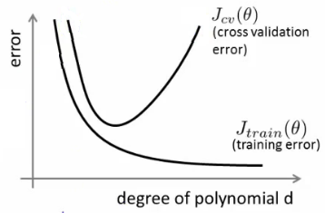
High Bias (Underfitting): Both training and cross-validation errors are high. The model is too simple and does not capture the underlying trend in the data well.
High Variance (Overfitting): Low training error but high cross-validation error. The model is too complex and captures noise in the training data, failing to generalize well.

Regularized Linear Regression Model

Consider a high-order polynomial linear regression model:

$$h_{\theta}(x) = \theta_0 + \theta_1x + \theta_2x^2 + \theta_3x^3 + \theta_4x^4$$

The regularized cost function for this model is:

$$J(\theta) = \frac{1}{2m} \left[ \sum_{i=1}^{m}(h_{\theta}(x^{(i)} - y^{(i)})^2 + \lambda \sum_{j=1}^{n} \theta_j^2 \right]$$

$\lambda$: Regularization parameter controlling the degree of regularization.
$\theta_j$: Coefficients of the polynomial terms.
$m$: Number of training examples.
$n$: Number of features (polynomial terms in this case).

Impact of the Regularization Parameter ($\lambda$)

The choice of $\lambda$ has a significant impact on the model's performance:

High $\lambda$ (High Bias): Leads to underfitting as it overly penalizes the coefficients, resulting in a too simple model.
Intermediate $\lambda$: Balances between bias and variance, often yielding a well-performing model.
Small $\lambda$ (High Variance): Leads to overfitting as it does not sufficiently penalize the coefficients, allowing the model to fit too closely to the training data.

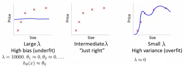
Effect of Lambda on Regularization

Try a range of $\lambda$ values, for each value minimize $J(\theta)$ to find $\theta^{(i)}$, and then compute the average squared error on the cross-validation set. Choose the $\lambda$ that results in the lowest error.

Learning Curves

Learning curves plot the training error and cross-validation error against the number of training examples. They help diagnose bias and variance issues.

Plotting Learning Curves:

$J_{train}$ (Training Error): Average squared error on the training set.
$J_{cv}$ (Cross-Validation Error): Average squared error on the cross-validation set.
$m$: Number of training examples.

Learning Curve Visualization

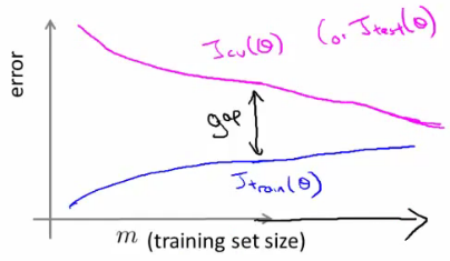
Small Training Sets: $J_{train}$ tends to be lower because the model can fit small datasets well.
As $m$ Increases: The model generalizes better, so $J_{cv}$ decreases.

Diagnosing Bias vs. Variance from Learning Curves

High Bias (Underfitting): Both $J_{train}$ and $J_{cv}$ are high, and adding more training data does not significantly improve performance.
High Variance (Overfitting): $J_{train}$ is low, but $J_{cv}$ is much higher. Increasing the training set size can help the model generalize better.

We'll use linear regression for simplicity, but the process can be adapted to other models, including logistic regression.

Here's the implementation:

import numpy as np
import matplotlib.pyplot as plt
from sklearn.linear_model import LogisticRegression
from sklearn.metrics import log_loss
from sklearn.model_selection import train_test_split

# Function to compute training and cross-validation errors
def learning_curves(X, y, X_val, y_val, model):
    m = len(y)
    train_errors = []
    val_errors = []
    
    for i in range(1, m + 1):
        # Train the model on the first i training examples
        model.fit(X[:i], y[:i])
        
        # Compute training error
        y_train_predict = model.predict_proba(X[:i])[:, 1]
        train_error = log_loss(y[:i], y_train_predict)
        train_errors.append(train_error)
        
        # Compute cross-validation error
        y_val_predict = model.predict_proba(X_val)[:, 1]
        val_error = log_loss(y_val, y_val_predict)
        val_errors.append(val_error)
    
    return train_errors, val_errors

# Plotting function
def plot_learning_curves(train_errors, val_errors):
    plt.plot(np.arange(1, len(train_errors) + 1), train_errors, label='Training Error')
    plt.plot(np.arange(1, len(train_errors) + 1), val_errors, label='Cross-Validation Error')
    plt.xlabel('Number of Training Examples')
    plt.ylabel('Error')
    plt.title('Learning Curves')
    plt.legend()
    plt.grid(True)
    plt.show()

# Example usage
if __name__ == "__main__":
    # Sample data (features and labels)
    X = np.array([[0.5, 1.5],
                  [1.5, 0.5],
                  [3, 3.5],
                  [2, 2.5],
                  [1, 1],
                  [3.5, 4],
                  [2.5, 3],
                  [1, 0.5]])
    y = np.array([0, 0, 1, 1, 2, 2, 1, 0])  # 0: Triangle, 1: Cross, 2: Square
    
    # Binary classification for simplicity (convert multi-class to binary problem)
    y_binary = (y == 1).astype(int)
    
    # Split data into training and cross-validation sets
    X_train, X_val, y_train, y_val = train_test_split(X, y_binary, test_size=0.3, random_state=42)
    
    # Initialize the logistic regression model
    model = LogisticRegression()
    
    # Compute learning curves
    train_errors, val_errors = learning_curves(X_train, y_train, X_val, y_val, model)
    
    # Plot learning curves
    plot_learning_curves(train_errors, val_errors)

Reference

These notes are based on the free video lectures offered by Stanford University, led by Professor Andrew Ng. These lectures are part of the renowned Machine Learning course available on Coursera. For more information and to access the full course, visit the Coursera course page.