Last modified: September 17, 2023
This article is written in: 🇺🇸
Neural Networks: Learning and Classification
Neural networks, a core algorithm in machine learning, draw inspiration from the human brain's structure and function. They consist of layers containing interconnected nodes (neurons), each designed to perform specific computational tasks. Neural networks can tackle various classification problems, such as binary and multi-class classifications. The efficacy of these networks is enhanced through the adjustment of their parameters, guided by a cost function that quantifies the deviation between predictions and actual values.
Classification Problems in Neural Networks
- Training Set Representation: Typically represented as ${(x^1, y^1), (x^2, y^2), ..., (x^n, y^n)}$, where $x^i$ is the $i^{th}$ input and $y^i$ is the corresponding target output.
- $L$: Total number of layers in the network.
- $s_l$: Number of units (excluding the bias unit) in layer $l$.
Example Network Architecture

In the illustrated network:
- There are 4 layers ($L=4$).
- The first layer ($s_1$) has 3 units.
- The second and third layers ($s_2$, $s_3$) each have 5 units.
- The fourth layer ($s_4$) has 4 units.
Binary Classification
In binary classification, the neural network predicts a single output which can take one of two possible values (often represented as 0 or 1). Characteristics of binary classification in neural networks include:
- Single Output Node: The final layer produces a real number value, interpreted as a probability or classification decision.
- Output Representation: $k = 1$ (one output class) and $s_L = 1$ (one unit in the output layer).
Multi-class Classification
Multi-class classification extends the network's capability to differentiate between multiple classes. Here, the target output $y$ is a vector representing the probability of each class. Characteristics include:
- Multiple Output Classes: $k$ distinct classifications are represented.
- Output Vector: The output $y$ is a $k$-dimensional vector of real numbers, where each element corresponds to a class.
- Layer Configuration: The output layer has $s_L = k$ units, each corresponding to one of the $k$ classes.
Learning Process
The learning process in neural networks involves:
- Cost Function: A generalization of the logistic regression cost function, which sums the error over all output units and classes. This function quantifies the difference between predicted and actual values.
- Gradient Computation: Employing the chain rule to calculate the partial derivatives of the cost function with respect to each network parameter.
- Backpropagation Algorithm: Used for efficiently computing these partial derivatives. The algorithm propagates the error signal backwards through the network, adjusting the parameters (weights and biases) to minimize the cost function.
Neural Network Cost Function
The cost function for neural networks is an extension of the logistic regression cost function, adapted for multiple outputs. This function evaluates the performance of a neural network by measuring the difference between the predicted outputs and the actual values across all output units.
The cost function for a neural network with multiple outputs (where $K$ is the number of output units) is defined as:
$$J(\Theta) = -\frac{1}{m} \sum_{i=1}^{m} \sum_{k=1}^{K}[ y_k^{(i)} \log{(h_{\Theta}(x^{(i)}))}k + (1- y_k^{(i)}) \log(1 - {(h{\Theta} (x^{(i)}))}k)] + \frac{\lambda}{2m} \sum{l=1}^{L-1} \sum_{i=1}^{s_l} \sum_{j=1}^{s_{l+1}} (\Theta^{(l)}_{ji})^2$$
- $m$: Number of training examples.
- $K$: Number of output units.
- $L$: Total number of layers in the network.
- $s_l$: Number of units in layer $l$.
- $y_k^{(i)}$: Actual value of the $k^{th}$ output unit for the $i^{th}$ training example.
- $h_{\Theta}(x^{(i)})$: Hypothesis function applied to the $i^{th}$ training example.
- $\lambda$: Regularization parameter to avoid overfitting.
- $\Theta^{(l)}_{ji}$: Weight from unit $i$ in layer $l$ to unit $j$ in layer $l+1$.
This function incorporates a sum over the $K$ output units for each training example, and also includes a regularization term to penalize large weights and prevent overfitting.
Partial Derivative Terms
In order to optimize the cost function, we need to understand how changes in the weights $\Theta$ affect the cost. This is where the partial derivative terms come into play.
- $\Theta^{(1)}_{ji}$: Represents the weight from the $i^{th}$ unit in layer 1 to the $j^{th}$ unit in layer 2.
- $\Theta^{(1)}{10}$ , $\Theta^{(1)}{11}$ , $\Theta^{(1)}_{21}$: Specific weights that map from the input layer to the first and second units in the second layer, including the bias unit.
Gradient Computation
Gradient computation in neural networks is achieved through a process known as backpropagation, which calculates the gradient of the cost function with respect to each weight in the network.
Forward Propagation Example
Consider a neural network with one training example $(x,y)$:
- Layer 1 (Input Layer): $a^{(1)} = x$ and $z^{(2)} = \Theta^{(1)}a^{(1)}$.
- Layer 2 (Hidden Layer): $a^{(2)} = g(z^{(2)})$, append $a^{(2)}_0$, and then $z^{(3)} = \Theta^{(2)}a^{(2)}$.
- Layer 3 (Another Hidden Layer): $a^{(3)} = g(z^{(3)})$, append $a^{(3)}_0$, and then $z^{(4)} = \Theta^{(3)}a^{(3)}$.
- Output Layer: $a^{(4)} = h_{\Theta}(x) = g(z^{(4)})$.

Each layer's output ($a^{(l)}$) becomes the input for the next layer, with the activation function $g$ (typically a sigmoid or ReLU function) applied to the weighted sums. The final output $a^{(4)}$ is the hypothesis of the network for the given input $x$. The backpropagation algorithm then computes the gradient by propagating the error backwards from the output layer to the input layer, adjusting the weights $\Theta$ to minimize the cost function $J(\Theta)$.
Backpropagation Algorithm
Backpropagation is a key algorithm in training neural networks, used for calculating the gradient of the cost function with respect to each parameter in the network. It involves propagating errors backward through the network, from the output layer to the input layer.
Calculating Error Terms (Deltas)
- $\delta_j$ Vector: Represents the error for each node $j$ in layer $l$. It is an $L \times 1$ vector, where $L$ is the total number of layers.
- Last Layer Error ($\delta^{(L)}$): For the last layer, the error is calculated as the difference between the network's output ($a^{(L)}$) and the actual value ($y$):
$$\delta^{(L)}_j = a^{(L)}_j - y_j$$
- Error for Other Layers: The error terms for the other layers are computed recursively using the errors from the subsequent layer:
$$\delta^{(l)}_j = (\Theta^{(l)}_j)^T \delta^{(l+1)} \cdot g'(z^{(l)}_j)$$
Accumulating Gradient ($\Delta$)
- Partial Derivative Accumulation: $\Delta^{(l)}{ij}$ accumulates the partial derivatives of the cost function with respect to the weights $\Theta^{(l)}{ij}$ :
$$\Delta^{(l)}{ij} = \Delta^{(l)}{ij} + a^{(l)}_j \delta^{(l+1)}_i$$
- Layer Notation: $l$ denotes the layer, $j$ the node in layer $l$, and $i$ the error of the affected node in the subsequent layer $l+1$.
Calculating the Gradient
The gradient of the cost function $J(\Theta)$ with respect to the weights is given by:
$$ \frac{\partial}{\partial \Theta^{(l)}{ij}}J(\Theta) = \begin{cases} \frac{1}{m} \Delta^{(l)}{ij} + \lambda \Theta ^{(l)}{ij} \quad &\text{if} \, j \neq 0 \\ \frac{1}{m} \Delta^{(l)}{ij} \quad &\text{if} \, j=0 \\ \end{cases} $$
Here's a Python implementation of the backpropagation algorithm using mock data. We will use NumPy to handle matrix operations and simulate the forward and backward passes through a neural network.
import numpy as np

# Mock data and network parameters
np.random.seed(42)
input_size = 3    # Number of input features
hidden_size = 5   # Number of hidden units
output_size = 2   # Number of output units
m = 10            # Number of training examples
lambda_reg = 0.01 # Regularization parameter

# Generate some random mock data
X = np.random.rand(m, input_size)
y = np.random.rand(m, output_size)

# Initialize weights randomly
Theta1 = np.random.rand(hidden_size, input_size + 1)
Theta2 = np.random.rand(output_size, hidden_size + 1)

# Sigmoid activation function
def sigmoid(z):
    return 1 / (1 + np.exp(-z))

# Derivative of sigmoid
def sigmoid_gradient(z):
    return sigmoid(z) * (1 - sigmoid(z))

# Add bias unit to input layer
X_bias = np.c_[np.ones((m, 1)), X]

# Forward pass
z2 = X_bias.dot(Theta1.T)
a2 = sigmoid(z2)
a2_bias = np.c_[np.ones((a2.shape[0], 1)), a2]
z3 = a2_bias.dot(Theta2.T)
a3 = sigmoid(z3)

# Calculate error terms (deltas)
delta3 = a3 - y
delta2 = delta3.dot(Theta2[:, 1:]) * sigmoid_gradient(z2)

# Accumulate gradients
Delta1 = np.zeros(Theta1.shape)
Delta2 = np.zeros(Theta2.shape)

for i in range(m):
    Delta1 += np.outer(delta2[i], X_bias[i])
    Delta2 += np.outer(delta3[i], a2_bias[i])

# Calculate the gradient
Theta1_grad = (1/m) * Delta1
Theta2_grad = (1/m) * Delta2

# Add regularization term
Theta1_grad[:, 1:] += (lambda_reg / m) * Theta1[:, 1:]
Theta2_grad[:, 1:] += (lambda_reg / m) * Theta2[:, 1:]

print("Gradient for Theta1:", Theta1_grad)
print("Gradient for Theta2:", Theta2_grad)- Backpropagation involves propagating errors backward through the network, starting from the output layer and moving to the input layer.
- Error terms, also known as deltas, are computed for each node in each layer of the network.
- For the last layer, the error is calculated as the difference between the network's output and the actual target value.
- Errors for other layers are computed recursively using the errors from the subsequent layer and the derivative of the activation function.
- The process of accumulating gradients involves calculating partial derivatives of the cost function with respect to the network's weights.
- These partial derivatives are accumulated over all training examples to compute the total gradient.
- The gradient of the cost function with respect to the weights is adjusted by averaging over the training examples and incorporating a regularization term to prevent overfitting.
- Regularization helps improve the generalization of the neural network by penalizing large weights.
Here is the expected output for the code provided above:
Gradient for Theta1: [[0.16460127 0.09018903 0.10866451 0.07285257]
                      [0.17977638 0.10320301 0.11857247 0.07947471]
                      [0.11092262 0.06493514 0.07037884 0.04835915]
                      [0.13438568 0.07016218 0.08659204 0.05121289]
                      [0.17372409 0.08792393 0.11033074 0.06408053]]
Gradient for Theta2: [[0.36423865 0.2588335  0.27099399 0.2588335  0.27099399 0.21043443]
                      [0.33764582 0.23963147 0.24547491 0.23963147 0.24547491 0.19303788]]
Gradient Checking
Due to the complexity of backpropagation, implementing it correctly is crucial. Gradient checking is a technique to validate the correctness of the computed gradients.
Steps in Gradient Checking:
- Function $J(\Theta)$: Start with a function representing the cost.
- Compute Perturbed Weights: Calculate $J(\Theta + \epsilon)$ and $J(\Theta - \epsilon)$, where $\epsilon$ is a small value.
- Slope Estimation: The derivative is approximated by the slope of the straight line joining these two points.
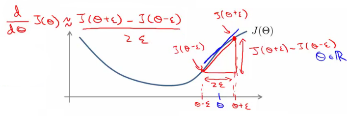
Gradient checking serves as a diagnostic tool to ensure that the backpropagation implementation is correct. However, it's computationally expensive and typically used only for debugging and not during regular training.
Reference
These notes are based on the free video lectures offered by Stanford University, led by Professor Andrew Ng. These lectures are part of the renowned Machine Learning course available on Coursera. For more information and to access the full course, visit the Coursera course page.