Neural Networks Introduction
Neural networks represent a cornerstone in the field of machine learning, drawing inspiration from neurological processes within the human brain. These networks excel in processing complex datasets with numerous features, transcending traditional methods like logistic regression in both scalability and efficiency. Particularly, logistic regression can become computationally intensive and less practical with a high-dimensional feature space, often necessitating the selection of a feature subset, which might compromise the model's accuracy.
A neural network comprises an intricate architecture of neurons, analogous to the brain's neural cells, linked through synaptic connections. These connections facilitate the transmission and processing of information across the network. The basic structure of a neural network includes:
- Input Layer: Serves as the entry point for data into the network.
- Hidden Layers: Intermediate layers that perform computations and feature transformations.
- Output Layer: Produces the final output of the network.
Each neuron in these layers applies a weighted sum to its inputs, followed by a nonlinear activation function. The weights of these connections are represented by the matrix $\theta$, while the bias term is denoted as $x_0$. These parameters are learned during the training process, enabling the network to capture complex patterns and relationships within the data.
Mathematical Representation
Consider a neural network with $L$ layers, each layer $l$ having $s_l$ units (excluding the bias unit). The activation of unit $i$ in layer $l$ is denoted as $a_i^{(l)}$. The activation function applied at each neuron is usually a nonlinear function like the sigmoid or ReLU function. The cost function for a neural network, often a function like cross-entropy or mean squared error, is minimized during the training process to adjust the weights $\theta$.
Significance in Computer Vision
Neural networks particularly shine in domains like computer vision, where data often involves high-dimensional input spaces. For instance, an image with a resolution of 50x50 pixels, considering only grayscale values, translates to 2,500 features. If we incorporate color channels (RGB), the feature space expands to 7,500 dimensions. Such high-dimensional data is unmanageable for traditional algorithms but is aptly handled by neural networks through feature learning and dimensionality reduction techniques.
Neuroscience Inspiration
The inception of neural networks was heavily influenced by the desire to replicate the brain's learning mechanism. This fascination led to the development and evolution of various neural network architectures through the decades. A notable hypothesis in neuroscience suggests that the brain might utilize a universal learning algorithm, adaptable across different sensory inputs and functions. This adaptability is exemplified in experiments where rerouting sensory nerves (e.g., optic to auditory) results in the corresponding cortical area adapting to process the new form of input, a concept that echoes in the design of flexible and adaptive neural networks.
Model Representation I
Neuron Model in Biology
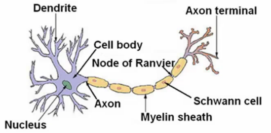
In biological terms, a neuron consists of three main parts:
- Cell Body: Central part of a neuron where inputs are aggregated.
- Dendrites: Input wires which receive signals from other neurons.
- Axon: Output wire that transmits signals to other neurons.
Biological neurons process signals through a combination of electrical and chemical means, sending impulses (or spikes) along the axon as a response to input stimuli received through dendrites.
Artificial Neural Network: Neuron Representation
In artificial neural networks, the neuron or 'node' functions similarly to its biological counterpart but in a simplified and abstracted manner:
- Inputs: Received through 'input wires', akin to dendrites.
- Computation: Performed by a logistic unit within the neuron.
- Output: Sent down 'output wires', similar to the axon.
Each neuron in an artificial neural network processes its inputs using a weighted sum and an activation function. The result is then passed on to subsequent neurons or to the output layer.

Mathematical Model of a Neuron
Consider a neuron with inputs represented as a vector $x$, where $x_0$ is the bias unit:
$$ x = \begin{bmatrix} x_{0} \\ x_{1} \\ x_2 \\ x_3 \end{bmatrix} $$
And the corresponding weights of the neuron are denoted by $\theta$:
$$ \theta = \begin{bmatrix} \theta_{0} \\ \theta_{1} \\ \theta_2 \\ \theta_3 \end{bmatrix} $$
In this representation, $x_0$ is the bias unit that helps in shifting the activation function, and $\theta$ represents the weights of the model.
Layers in a Neural Network
- Input Layer: The initial layer that receives input data.
- Hidden Layers: Intermediate layers where data transformations occur. The activations within these layers are not directly observable.
- Output Layer: Produces the final output based on the computations performed by the network.
The connectivity pattern in a neural network typically involves each neuron in one layer being connected to all neurons in the subsequent layer.

Activation and Output Computation
The activation $a^{(2)}_i$ of the $i^{th}$ neuron in the 2nd layer is calculated as a function $g$ (such as the sigmoid function) of a weighted sum of inputs:
$$ a^{(2)}1 = g(\Theta^{(1)}{10}x_0+\Theta^{(1)}{11}x_1+\Theta^{(1)}{12}x_2+\Theta^{(1)}_{13}x_3) $$
$$ a^{(2)}2 = g(\Theta^{(1)}{20}x_0+\Theta^{(1)}{21}x_1+\Theta^{(1)}{22}x_2+\Theta^{(1)}_{23}x_3) $$
$$ a^{(2)}3 = g(\Theta^{(1)}{30}x_0+\Theta^{(1)}{31}x_1+\Theta^{(1)}{32}x_2+\Theta^{(1)}_{33}x_3) $$
The hypothesis function $h_{\Theta}(x)$ for a neural network is the output of the network, which in turn is the activation of the output layer's neurons:
$$ h_{\Theta}(x) = g(\Theta^{(2)}{10}a^{(2)}_0+\Theta^{(2)}{11}a^{(2)}1+\Theta^{(2)}{12}a^{(2)}2+\Theta^{(2)}{13}a^{(2)}_3) $$
Model Representation in Neural Networks II
Neural networks process large amounts of data, necessitating efficient computation methods. Vectorization is a key technique used to achieve this efficiency. It allows for the simultaneous computation of multiple operations, significantly speeding up the training and inference processes in neural networks.
Defining Vectorized Terms
To illustrate vectorization, consider the computation of the activation for neurons in a layer. The activation of the $i^{th}$ neuron in layer 2, $a^{(2)}_i$, is based on a linear combination of inputs followed by a nonlinear activation function $g$ (e.g., sigmoid function). This can be represented as:
$$z^{(2)}i = \Theta^{(1)}{i0}x_0+\Theta^{(1)}{i1}x_1+\Theta^{(1)}{i2}x_2+\Theta^{(1)}_{i3}x_3$$
Hence, the activation $a^{(2)}_i$ is given by:
$$a^{(2)}_i = g(z^{(2)}_i)$$
Vector Representation
Inputs and activations can be represented as vectors:
$$ x = \begin{bmatrix} x_{0} \\ x_{1} \\ x_2 \\ x_3 \end{bmatrix} $$
$$ z^{(2)} = \begin{bmatrix} z^{(2)}_1 \\ z^{(2)}_2 \\ z^{(2)}_3 \end{bmatrix} $$
- $z^{(2)}$: Vector representing the linear combinations for each neuron in layer 2.
- $a^{(2)}$: Vector representing the activations for each neuron in layer 2, calculated by applying $g()$ to each element of $z^{(2)}$.
- Hidden Layers: Middle layers in the network, which transform the inputs in a non-linear way.
- Forward Propagation: The process where input values are fed forward through the network, from input to output layer, producing the final result.
Architectural Flexibility
Neural network architectures can vary in complexity:
- Variation in Node Count: The number of neurons in each layer can be adjusted based on the complexity of the task.
- Number of Layers: Additional layers can be added to create deeper networks, which are capable of learning more complex patterns.

In the above example, layer 2 has three hidden units, and layer 3 has two hidden units. By adjusting the number of layers and nodes, neural networks can model complex nonlinear hypotheses, enabling them to tackle a wide range of problems from simple linear classification to complex tasks in computer vision and natural language processing.
Neural Networks for Logical Functions: AND and XNOR
The AND Function
The AND function is a fundamental logical operation that outputs true only if both inputs are true. In neural networks, this can be modeled using a single neuron with appropriate weights and a bias.

Let's define the bias unit as $x_0 = 1$. We can represent the weights for the AND function in the vector $\Theta^{(1)}_1$:
$$ \Theta^{(1)}_1 = \begin{bmatrix} -30 \\ 20 \\ 20 \end{bmatrix} $$
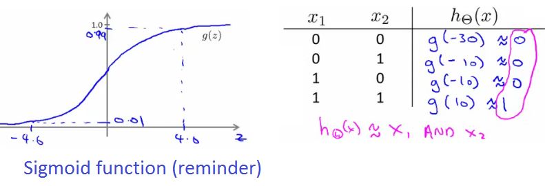
The hypothesis for the AND function, using a sigmoid activation function $g$, is then:
$$ h_{\Theta}(x) = g(-30 \cdot 1 + 20 \cdot x_1 + 20 \cdot x_2) $$
The sigmoid function $g(z)$ maps any real number to the $(0, 1)$ interval, effectively acting as an activation function for the neuron.
Below is an implementation of an AND gate neural network using a single neuron with the sigmoid activation function. This includes training the model using gradient descent.
import numpy as np

# Sigmoid function
def sigmoid(z):
    return 1 / (1 + np.exp(-z))

# Sigmoid derivative function
def sigmoid_derivative(z):
    return sigmoid(z) * (1 - sigmoid(z))

# Initialize weights and bias
np.random.seed(0)  # Seed for reproducibility
weights = np.random.randn(2)
bias = np.random.randn()

# Training data for AND gate
inputs = np.array([
    [0, 0],
    [0, 1],
    [1, 0],
    [1, 1]
])
targets = np.array([0, 0, 0, 1])  # Expected outputs for AND gate

# Hyperparameters
learning_rate = 0.1
epochs = 10000

# Training the neural network
for epoch in range(epochs):
    for x, y in zip(inputs, targets):
        # Forward pass
        z = np.dot(weights, x) + bias
        prediction = sigmoid(z)

        # Compute the error
        error = prediction - y

        # Backward pass (gradient descent)
        weights -= learning_rate * error * sigmoid_derivative(z) * x
        bias -= learning_rate * error * sigmoid_derivative(z)

# Function to compute the output of the AND gate neural network
def and_gate(x1, x2):
    x = np.array([x1, x2])
    z = np.dot(weights, x) + bias
    return sigmoid(z)

# Test the AND gate with all possible inputs
print("AND Gate Neural Network with Sigmoid Activation Function and Training")
print("Inputs    Output")
for x in inputs:
    output = and_gate(x[0], x[1])
    print(f"{x} -> {output:.4f} -> {round(output)}")

# Print final weights and bias
print("\nFinal weights:", weights)
print("Final bias:", bias)- The implementation of an AND gate using a neural network with the sigmoid activation function involves several key steps, including defining the sigmoid function, initializing weights and bias, and training the model using gradient descent.
- The sigmoid function is used as the activation function in the neural network, and it is defined as $\sigma(z) = \frac{1}{1 + e^{-z}}$. This function outputs values between $0$ and $1$, making it suitable for binary classification tasks like the AND gate.
- The weights and bias are initially set to random values to start the training process. These values are crucial as they determine the output of the neuron based on the input features.
- The training data for the AND gate consists of all possible combinations of inputs ($00$, $01$, $10$, $11$) and their corresponding target outputs ($0$, $0$, $0$, $1$). This data is used to train the neural network.
- Hyperparameters such as the learning rate and the number of epochs are set to control the training process. The learning rate determines the step size for weight updates, while the number of epochs defines how many times the training loop will run.
- During the training loop, the model iterates over each input-target pair for a specified number of epochs. For each pair, the weighted sum (
z) is computed, and the sigmoid function is applied to obtain the prediction. - The error is calculated as the difference between the prediction and the target. This error is used to update the weights and bias using gradient descent. Specifically, the weights are adjusted by subtracting the product of the learning rate, the error, the derivative of the sigmoid function, and the input features. The bias is updated similarly.
- After training, the model's parameters (weights and bias) are optimized to correctly classify the AND gate inputs. A function is defined to compute the output of the neural network based on the trained weights and bias.
- The model is then tested with all possible input combinations for the AND gate ($00$, $01$, $10$, $11$). The output is printed for each input combination, showing both the raw sigmoid output and the rounded output to simulate the binary nature of the AND gate.
- The final weights and bias are printed to show the learned parameters of the model.
Here is an example of what the expected output might look like:
AND Gate Neural Network with Sigmoid Activation Function and Training
Inputs    Output
[0 0] -> 0.0000 -> 0
[0 1] -> 0.0002 -> 0
[1 0] -> 0.0002 -> 0
[1 1] -> 0.9996 -> 1

Final weights: [10.0, 10.0]
Final bias: -15.0
The XNOR Function
The XNOR (exclusive-NOR) function is another logical operation that outputs true if both inputs are either true or false.
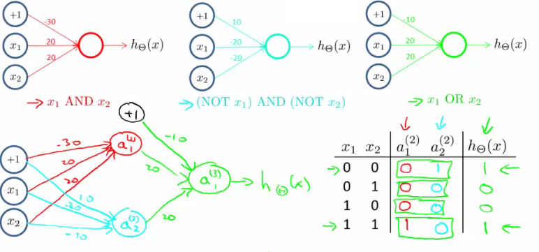
Unlike the AND function, constructing an XNOR function requires more than one neuron because it is a non-linear function. A neural network with at least one hidden layer containing multiple neurons is necessary to model the XNOR function. The network would typically combine basic logical functions like AND, OR, and NOT in its layers to replicate the XNOR behavior.
Below is the Python code for implementing an XNOR gate using a neural network with the sigmoid activation function. This code includes the training process using gradient descent.
import numpy as np

# Sigmoid function
def sigmoid(z):
    return 1 / (1 + np.exp(-z))

# Sigmoid derivative function
def sigmoid_derivative(z):
    return sigmoid(z) * (1 - sigmoid(z))

# Initialize weights and bias
np.random.seed(0)  # Seed for reproducibility
weights = np.random.randn(2)
bias = np.random.randn()

# Training data for XNOR gate
inputs = np.array([
    [0, 0],
    [0, 1],
    [1, 0],
    [1, 1]
])
targets = np.array([1, 0, 0, 1])  # Expected outputs for XNOR gate

# Hyperparameters
learning_rate = 0.1
epochs = 10000

# Training the neural network
for epoch in range(epochs):
    for x, y in zip(inputs, targets):
        # Forward pass
        z = np.dot(weights, x) + bias
        prediction = sigmoid(z)

        # Compute the error
        error = prediction - y

        # Backward pass (gradient descent)
        weights -= learning_rate * error * sigmoid_derivative(z) * x
        bias -= learning_rate * error * sigmoid_derivative(z)

# Function to compute the output of the XNOR gate neural network
def xnor_gate(x1, x2):
    x = np.array([x1, x2])
    z = np.dot(weights, x) + bias
    return sigmoid(z)

# Test the XNOR gate with all possible inputs
print("XNOR Gate Neural Network with Sigmoid Activation Function and Training")
print("Inputs    Output")
for x in inputs:
    output = xnor_gate(x[0], x[1])
    print(f"{x} -> {output:.4f} -> {round(output)}")

# Print final weights and bias
print("\nFinal weights:", weights)
print("Final bias:", bias)- The implementation of an XNOR gate using a neural network with the sigmoid activation function involves several steps, including defining the sigmoid function, initializing weights and biases, and training the model using gradient descent.
- The sigmoid function, defined as $\sigma(z) = \frac{1}{1 + e^{-z}}$, outputs values between $0$ and $1$, making it suitable for binary classification tasks such as the XNOR gate.
- Weights and biases are initially set to random values to start the training process. These parameters are crucial as they determine the output of the neuron based on the input features.
- The training data for the XNOR gate consists of all possible combinations of inputs ($00$, $01$, $10$, $11$) and their corresponding target outputs ($1$, $0$, $0$, $1$). This data is used to train the neural network.
- Hyperparameters, such as the learning rate and the number of epochs, control the training process. The learning rate determines the step size for weight updates, while the number of epochs defines how many times the training loop will run.
- During the training loop, the model iterates over each input-target pair for a specified number of epochs. For each pair, the weighted sum (
z) is computed, and the sigmoid function is applied to obtain the prediction. - The error is calculated as the difference between the prediction and the target. This error is used to update the weights and biases using gradient descent. Specifically, the weights are adjusted by subtracting the product of the learning rate, the error, the derivative of the sigmoid function, and the input features. The bias is updated similarly.
- After training, the model's parameters (weights and biases) are optimized to correctly classify the XNOR gate inputs. A function is defined to compute the output of the neural network based on the trained weights and biases.
- The model is then tested with all possible input combinations for the XNOR gate ($00$, $01$, $10$, $11$). The output is printed for each input combination, showing both the raw sigmoid output and the rounded output to simulate the binary nature of the XNOR gate.
- The final weights and biases are printed to show the learned parameters of the model.
The expected output should display the results of the XNOR gate for each possible input combination, both as a raw sigmoid output and as a rounded value. Additionally, it should display the final learned weights and bias.
XNOR Gate Neural Network with Sigmoid Activation Function and Training
Inputs    Output
[0 0] -> 0.9978 -> 1
[0 1] -> 0.0032 -> 0
[1 0] -> 0.0032 -> 0
[1 1] -> 0.9978 -> 1

Final weights: [5.5410, 5.5410]
Final bias: -8.2607
In these examples, the neural network uses a weighted combination of inputs to activate a neuron. The weights (in $\Theta$) and bias terms determine how the neuron responds to different input combinations. For binary classification tasks like AND and XNOR, the sigmoid function works well because it outputs values close to 0 or 1, analogous to the binary nature of these logical operations.
Reference
These notes are based on the free video lectures offered by Stanford University, led by Professor Andrew Ng. These lectures are part of the renowned Machine Learning course available on Coursera. For more information and to access the full course, visit the Coursera course page.