Regularization

Last modified: March 26, 2023

This article is written in: 🇺🇸

Regularization

Regularization is a technique used to prevent overfitting in machine learning models, ensuring they perform well not only on the training data but also on new, unseen data.

Overfitting in Machine Learning

Issue: A model might fit the training data too closely, capturing noise rather than the underlying pattern.
Effect: Poor performance on new data.
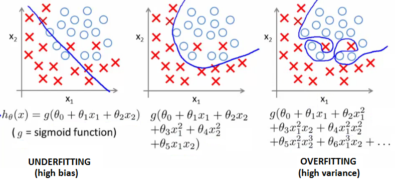
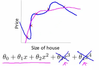
Manifestation in Regression: Occurs when using higher-degree polynomials which results in a high variance hypothesis.

Example: Overfitting in Logistic Regression

overfitting_logistic_regression

Regularization in Cost Function

Regularization works by adding a penalty term to the cost function that penalizes large coefficients, thereby reducing the complexity of the model.

Regularization in Linear Regression

Regularized Cost Function:

$min \frac{1}{2 m} [\sum_{i = 1}^{m} (h_{θ} (x^{(i)}) - y^{(i)})^{2} + λ \sum_{j = 1}^{m} θ_{j}^{2}]$

Penalization: Large values of $θ_{3}$ and $θ_{4}$ are penalized, leading to simpler models.

optimization_regularization

Regularization Parameter: $λ$

Role of $λ$ : Controls the trade-off between fitting the training set well and keeping the model simple (smaller parameter values).
Selection: Automated methods can be used to choose an appropriate $λ$ .

Modifying Gradient Descent

The gradient descent algorithm can be adjusted to include the regularization term:

I. For $θ_{0}$ (no regularization):

$\frac{\partial}{\partial θ_{0}} J (θ) = \frac{1}{m} \sum_{i = 1}^{m} (h_{θ} (x^{(i)}) - y^{(i)}) x_{0}^{(i)}$

II. For $θ_{j}$ ( $j \geq 1$ ):

$\frac{\partial}{\partial θ_{j}} J (θ) = (\frac{1}{m} \sum_{i = 1}^{m} (h_{θ} (x^{(i)}) - y^{(i)}) x_{j}^{(i)}) + \frac{λ}{m} θ_{j}$

Regularized Linear Regression

Regularized linear regression incorporates a regularization term in the cost function and its optimization to control model complexity and prevent overfitting.

Gradient Descent with Regularization

To optimize the regularized linear regression model using gradient descent, the algorithm is adjusted as follows:

while not converged:
  for j in [0, ..., n]:
      θ_j := θ_j - α [ \frac{1}{m} \sum_{i=1}^{m}(h_{θ}(x^{(i)}) + y^{(i)})x_j^{(i)} + \frac{λ}{m} θ_j ]

Here is the Python code to demonstrate regularization in linear regression, including the regularized cost function and gradient descent with regularization. This example uses numpy to implement the regularized linear regression model:

import numpy as np

def hypothesis(X, theta):
    return np.dot(X, theta)

def compute_cost(X, y, theta, lambda_reg):
    m = len(y)
    h = hypothesis(X, theta)
    cost = (1 / (2 * m)) * (np.sum((h - y) ** 2) + lambda_reg * np.sum(theta[1:] ** 2))
    return cost

def gradient_descent(X, y, theta, alpha, lambda_reg, num_iters):
    m = len(y)
    cost_history = np.zeros(num_iters)

    for iter in range(num_iters):
        h = hypothesis(X, theta)
        theta[0] = theta[0] - alpha * (1 / m) * np.sum((h - y) * X[:, 0])
        for j in range(1, len(theta)):
            theta[j] = theta[j] - alpha * ((1 / m) * np.sum((h - y) * X[:, j]) + (lambda_reg / m) * theta[j])
        
        cost_history[iter] = compute_cost(X, y, theta, lambda_reg)

    return theta, cost_history

# Example usage with mock data
np.random.seed(42)
X = np.random.rand(10, 2)  # Feature matrix (10 examples, 2 features)
y = np.random.rand(10)     # Target values

# Adding a column of ones to X for the intercept term (theta_0)
X = np.hstack((np.ones((X.shape[0], 1)), X))

# Initial parameters
theta = np.random.randn(X.shape[1])
alpha = 0.01  # Learning rate
lambda_reg = 0.1  # Regularization parameter
num_iters = 1000  # Number of iterations

# Perform gradient descent with regularization
theta, cost_history = gradient_descent(X, y, theta, alpha, lambda_reg, num_iters)

print("Optimized parameters:", theta)
print("Final cost:", cost_history[-1])

Regularization with the Normal Equation

In the normal equation approach for regularized linear regression, the optimal $θ$ is computed as follows:

regularized_normal_equation

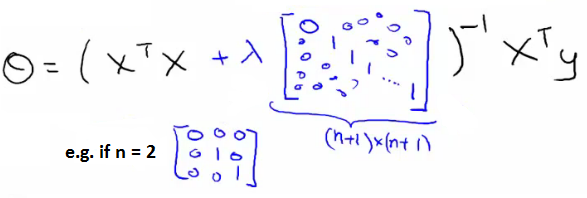
The equation includes an additional term $λ I$ to the matrix being inverted, ensuring regularization is accounted for in the solution.

Here is the Python code to implement regularized linear regression using the normal equation:

import numpy as np

def regularized_normal_equation(X, y, lambda_reg):
    m, n = X.shape
    I = np.eye(n)
    I[0, 0] = 0  # Do not regularize the bias term (theta_0)
    
    theta = np.linalg.inv(X.T @ X + lambda_reg * I) @ X.T @ y
    return theta

# Example usage with mock data
np.random.seed(42)
X = np.random.rand(10, 2)  # Feature matrix (10 examples, 2 features)
y = np.random.rand(10)     # Target values

# Adding a column of ones to X for the intercept term (theta_0)
X = np.hstack((np.ones((X.shape[0], 1)), X))

# Regularization parameter
lambda_reg = 0.1

# Compute the optimal parameters using the regularized normal equation
theta = regularized_normal_equation(X, y, lambda_reg)

print("Optimized parameters using regularized normal equation:", theta)

Regularized Logistic Regression

The cost function for logistic regression with regularization is:

$J (θ) = \frac{1}{m} \sum_{i = 1}^{m} [- y^{(i)} \log (h_{θ} (x^{(i)})) - (1 - y^{(i)}) \log (1 - h_{θ} (x^{(i)}))] + \frac{λ}{2 m} \sum_{j = 1}^{n} θ_{j}^{2}$

Gradient of the Cost Function

The gradient is defined for each parameter $θ_{j}$ :

I. For $j = 0$ (no regularization on $θ_{0}$ ):

$\frac{\partial}{\partial θ_{0}} J (θ) = \frac{1}{m} \sum_{i = 1}^{m} (h_{θ} (x^{(i)}) - y^{(i)}) x_{j}^{(i)}$

II. For $j \geq 1$ (includes regularization):

$\frac{\partial}{\partial θ_{j}} J (θ) = (\frac{1}{m} \sum_{i = 1}^{m} (h_{θ} (x^{(i)}) - y^{(i)}) x_{j}^{(i)}) + \frac{λ}{m} θ_{j}$

Optimization

For both linear and logistic regression, the gradient descent algorithm is updated to include regularization:

while not converged:
  for j in [0, ..., n]:
      θ_j := θ_j - α [ \frac{1}{m} \sum_{i=1}^{m}(h_{θ}(x^{(i)}) + y^{(i)})x_j^{(i)} + \frac{λ}{m} θ_j ]

The key difference in logistic regression lies in the hypothesis function $h_{θ} (x)$ , which is based on the logistic (sigmoid) function.

Here is the Python code to implement regularized logistic regression using gradient descent:

import numpy as np
from scipy.special import expit  # Sigmoid function

def sigmoid(z):
    return expit(z)

def compute_cost(X, y, theta, lambda_reg):
    m = len(y)
    h = sigmoid(np.dot(X, theta))
    cost = (1 / m) * np.sum(-y * np.log(h) - (1 - y) * np.log(1 - h)) + (lambda_reg / (2 * m)) * np.sum(theta[1:] ** 2)
    return cost

def gradient_descent(X, y, theta, alpha, lambda_reg, num_iters):
    m = len(y)
    cost_history = np.zeros(num_iters)

    for iter in range(num_iters):
        h = sigmoid(np.dot(X, theta))
        error = h - y
        
        theta[0] = theta[0] - alpha * (1 / m) * np.sum(error * X[:, 0])
        for j in range(1, len(theta)):
            theta[j] = theta[j] - alpha * ((1 / m) * np.sum(error * X[:, j]) + (lambda_reg / m) * theta[j])
        
        cost_history[iter] = compute_cost(X, y, theta, lambda_reg)

    return theta, cost_history

# Example usage with mock data
np.random.seed(42)
X = np.random.rand(10, 2)  # Feature matrix (10 examples, 2 features)
y = np.random.randint(0, 2, 10)  # Binary target values

# Adding a column of ones to X for the intercept term (theta_0)
X = np.hstack((np.ones((X.shape[0], 1)), X))

# Initial parameters
theta = np.random.randn(X.shape[1])
alpha = 0.01  # Learning rate
lambda_reg = 0.1  # Regularization parameter
num_iters = 1000  # Number of iterations

# Perform gradient descent with regularization
theta, cost_history = gradient_descent(X, y, theta, alpha, lambda_reg, num_iters)

print("Optimized parameters:", theta)
print("Final cost:", cost_history[-1])

Reference

These notes are based on the free video lectures offered by Stanford University, led by Professor Andrew Ng. These lectures are part of the renowned Machine Learning course available on Coursera. For more information and to access the full course, visit the Coursera course page.

Regularization

Overfitting in Machine Learning

Example: Overfitting in Logistic Regression

Regularization in Cost Function

Regularization in Linear Regression

Regularization Parameter: λλ

Modifying Gradient Descent

Regularized Linear Regression

Gradient Descent with Regularization

Regularization with the Normal Equation

Regularized Logistic Regression

Gradient of the Cost Function

Optimization

Reference

Table of Contents

Related Articles

Regularization Parameter: $λ$