Large Scale Machine Learning

Training machine learning models on large datasets poses significant challenges due to the computational intensity involved. To effectively handle this, various techniques such as stochastic gradient descent and online learning are employed. Let's delve into these methods and understand how they facilitate large-scale learning.

Learning with Large Datasets

To achieve high performance, one effective approach is using a low bias algorithm on a massive dataset. For example:

• Scenario: Consider a dataset with m = 100,000,000 examples.
• Challenge: Training a model like logistic regression on this scale requires significant computation for each gradient descent step.

Logistic Regression Update Rule:

$$ \theta_j := \theta_j - \alpha \frac{1}{m} \sum_{i=1}^m(h_{\theta}(x^{(i)}) - y^{(i)}) x_j^{(i)} $$

• Approach: Experiment with a smaller sample (say, 1000 examples) to test performance.

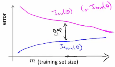
Diagnosing Bias vs. Variance:

• A large gap between training and cross-validation errors indicates high variance, suggesting more data might help.
• A small gap together with high loss can suggest underfitting after optimization and data quality are checked. A small gap at low loss can instead describe a useful model.

Stochastic Gradient Descent (SGD)

SGD optimizes the learning process for large datasets by updating parameters more frequently:

• Batch Gradient Descent: Traditional method that sums gradient terms over all examples before updating parameters. Its full-data pass can be costly, although vectorized or distributed batches can still be efficient when data and hardware permit.

• SGD Approach: Randomly shuffle the training examples. Update $\theta_j$ for each example:

$$ \theta_j := \theta_j - \alpha (h_{\theta}(x^{(i)}) - y^{(i)}) x_j^{(i)} $$

• This results in parameter updates for every training example, rather than at the end of a full pass over the data.

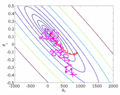
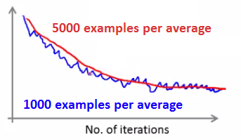
• Convergence Observation: Observe the cost function versus the number of iterations.

Online Learning

• Concept: Online learning is a dynamic form of learning where the model updates its parameters as new data arrives.
• Use Case: Ideal for continuously evolving datasets or when data comes in streams.
• Advantage: Allows the model to adapt to new trends or changes in the data over time.

Example: Product Search on a Cellphone Website

Imagine a cellphone-selling website scenario:

• User Queries: Users enter queries like "Android phone 1080p camera."
• Ranking Phones: The objective is to present the user with a list of ten phones, ranked according to their relevance or appeal.
• Feature Vectors: Generate a feature vector (x) for each phone, tailored to the user’s specific query.
• Click Prediction (CTR): Learn the probability $p(y = 1 | x; \theta)$, where $y = 1$ if a user clicks on a phone link, and $y = 0$ otherwise. This probability represents the predicted click-through rate (CTR).
• Utilizing CTR: Rank and display phones based on their estimated CTR, showing the most likely to be clicked options first.

Here's a mock implementation of a Online Learning using Python:

Step 1: Data Collection

Collect data on user queries and clicks on phone links. For simplicity, let's assume the data looks like this:

Step 2: Feature Extraction

Extract feature vectors for each phone based on user queries. These features can include attributes like price, camera quality, battery life, etc.

Step 3: Model Initialization

Initialize a simple logistic regression model for CTR prediction:

from sklearn.linear_model import SGDClassifier
import numpy as np

# Initialize the model
model = SGDClassifier(loss='log_loss', learning_rate='constant', eta0=0.01, random_state=0)

# Assume initial training data (for illustration purposes)
X_initial = np.array([[0.8, 0.2, 0.9, 0.4], [0.6, 0.4, 0.8, 0.5], [0.3, 0.9, 0.5, 0.7]])
y_initial = np.array([1, 0, 1])

# Initial training
model.partial_fit(X_initial, y_initial, classes=np.array([0, 1]))

Step 4: Online Learning Process

Update the model with new data as it arrives:

def update_model(new_data):
    X_new = np.array([data['features'] for data in new_data])
    y_new = np.array([data['click'] for data in new_data])
    model.partial_fit(X_new, y_new)

# Example of new data arriving
new_data = [
    {'features': [0.7, 0.3, 0.85, 0.45], 'click': 1},
    {'features': [0.5, 0.5, 0.75, 0.55], 'click': 0},
]

# Update the model with new data
update_model(new_data)

Step 5: Ranking Phones

Predict the CTR for new user queries and rank the phones accordingly:

def rank_phones(phones):
    # Extract features for each phone based on the user query
    feature_vectors = [phone['features'] for phone in phones]
    # Predict CTR for each phone
    predicted_ctr = model.predict_proba(feature_vectors)[:, 1]
    # Rank phones by predicted CTR
    ranked_phones = sorted(zip(phones, predicted_ctr), key=lambda x: x[1], reverse=True)
    return ranked_phones[:10]

# Example phones data
phones = [
    {'id': 1, 'features': [0.8, 0.2, 0.9, 0.4]},
    {'id': 2, 'features': [0.6, 0.4, 0.8, 0.5]},
    {'id': 3, 'features': [0.3, 0.9, 0.5, 0.7]},
    # More phones...
]

# Rank phones for a given user query
top_phones = rank_phones(phones)
print(top_phones)

Map Reduce in Large Scale Machine Learning

Map Reduce is a programming model designed for processing large datasets across distributed clusters. It simplifies parallel computation on massive scales, making it a cornerstone for big data analytics and machine learning where traditional single-node processing falls short.

Understanding Map Reduce

Map Reduce works by breaking down the processing into two main phases: Map phase and Reduce phase.

I. Map Phase:

• Operation: This phase involves taking a large input and dividing it into smaller sub-problems. Each sub-problem is processed independently.
• Function: The map function applies a specific operation to each sub-problem. For example, it might involve filtering data or sorting it.
• Output: The result of the map function is a set of key-value pairs.

II. Reduce Phase:

• Operation: In this phase, the output from the map phase is combined or reduced into a smaller set of tuples.
• Function: The reduce function aggregates the results to form a consolidated output.
• Examples: Summation, counting, or averaging over large datasets.

Implement the Aggregation before Choosing a Distributed Runtime

For an average loss, each worker can return its example count, summed loss, and summed gradient at the same parameter vector. A reducer adds those quantities and divides by the total count. Unequal partitions therefore require count weighting; taking an unweighted mean of worker means defines another objective.

Hadoop Streaming can express map and reduce stages as processes exchanging keyed records. The important learning calculation is the reduction of loss and gradient sufficient summaries, rather than the presence of a particular cluster command. The executable NumPy example below verifies that reduction on one process, without claiming to launch a distributed system.

For iterative learning, workers also need the current shared parameters. Performing several local updates and then averaging the resulting parameter vectors is generally different from averaging gradients evaluated at one common point. Communication frequency, stale parameters, and data partitioning become part of the optimization method.

Advantages of Map Reduce

• Scalability: Can handle petabytes of data by distributing tasks across numerous machines.
• Fault Tolerance: Automatically handles failures. If a node fails, tasks are rerouted to other nodes.
• Flexibility: Capable of processing structured, semi-structured, and unstructured data.

Applications in Machine Learning

• Large-scale Data Processing: For training models on datasets that are too large for a single machine, especially for tasks like clustering, classification, and pattern recognition.
• Parallel Training: Training multiple models or model parameters in parallel, reducing the overall training time.
• Data Preprocessing: Large-scale data cleaning, transformation, and feature extraction.

Forms of Parallelization

• Multiple Machines: Distribute the data and computations across several machines.
• Multiple CPUs: Utilize several CPUs within a machine.
• Multiple Cores: Take advantage of multi-core processors for parallel processing.

Local and Distributed Parallelization

• Numerical Linear Algebra Libraries: Some libraries can automatically parallelize computations across multiple cores.
• Vectorization: With an efficient vectorization implementation, local libraries might handle much of the optimization, reducing the need for manual parallelization.
• Distributed Systems: For data that's too large for a single system, distributed computing frameworks like Hadoop are used. These frameworks apply the Map Reduce paradigm to process data across multiple machines.

Compute and Compare the Batch Gradients

For six inputs $x=(-1,-0.6,-0.2,0.2,0.6,1)$, let $y=1+2x$ and start intercept and slope at zero. The half-MSE gradient is $X^\top(X\theta-y)/6=(-1,-0.9333333)$.

Partition the first two observations onto one worker and the remaining four onto another. Their mean gradients are $(0.6,-0.56)$ and $(-1.8,-1.12)$. Weighting by their counts gives

$$ \frac{2(0.6,-0.56)+4(-1.8,-1.12)}6 =(-1,-0.9333333). $$

The unweighted mean is $(-0.6,-0.84)$ and does not match the full-data objective. The mismatch appears even with correct arithmetic on each worker.

import numpy as np
from sklearn.linear_model import LinearRegression, SGDRegressor
x = np.linspace(-1.0, 1.0, 6)
X = np.column_stack([np.ones(6), x])
y = 1 + 2 * x
theta = np.zeros(2)

def gradient(rows):
    return X[rows].T @ (X[rows] @ theta - y[rows]) / len(X[rows])
groups = [np.arange(2), np.arange(2, 6)]
full = gradient(np.arange(6))
weighted = sum((len(g) * gradient(g) for g in groups)) / len(X)
unweighted = np.mean([gradient(g) for g in groups], axis=0)
np.testing.assert_allclose(weighted, full)
assert not np.allclose(unweighted, full)
model = SGDRegressor(loss='squared_error', penalty=None, learning_rate='constant', eta0=0.02, random_state=0, shuffle=False)
for _ in range(600):
    for rows in groups:
        model.partial_fit(x[rows, None], y[rows])
reference = LinearRegression().fit(x[:, None], y)
np.testing.assert_allclose(model.predict(x[:, None]), reference.predict(x[:, None]), atol=1e-05)
print('full/weighted gradient:', np.round(full, 8), np.round(weighted, 8))
print('unweighted worker-mean gradient:', np.round(unweighted, 8))
print('streamed SGD intercept/slope:', np.round(model.intercept_, 6), np.round(model.coef_, 6))

The streaming estimator receives the same six observations through repeated partial-fit calls. In this noiseless fixture it converges to intercept one and slope two, matching a direct least-squares fit. That result checks the update interface on a simple problem; noisy data with a constant step size can continue fluctuating near an optimum.

Mini-Batch Size Trades Work per Update against Gradient Noise

For a uniform randomly sampled observation at a fixed parameter vector, its gradient is an unbiased estimate of the empirical mean gradient. Averaging a mini-batch can reduce its variance. Independent gradient draws would reduce covariance by the batch size, while related or without-replacement draws require their corresponding covariance calculation.

One full-data update, six sequential single-example updates, and two mini-batch updates are not identical: later updates use changed parameters. Epoch counts describe passes over data, while update counts describe parameter changes. Compare computational work and held-out performance rather than treating one update as a common unit across methods.

Shuffling helps prevent an ordering such as all negatives followed by all positives from dominating consecutive steps. A decreasing learning rate can reduce late optimization noise under suitable assumptions; an adaptive or constant rate may be useful when a changing process needs continuing adaptation. These are different objectives, and a learning-rate schedule alone does not guarantee convergence.

Count the Memory before Designing the Training Loop

A dense matrix with 100 million rows and 100 float64 features requires $10^8(100)(8)=80$ billion bytes, approximately 74.5 GiB, before labels, copies, and optimizer storage. A 256-row feature batch requires 204,800 bytes, or 200 KiB. The parameter vector is much smaller.

This difference motivates out-of-core reading, sparse features, or mini-batches when the full matrix does not fit. It does not eliminate preprocessing costs or the need to evaluate the model. A vectorized expression that accidentally creates all pairwise differences can allocate a much larger array than the intended batch.

For linear squared loss, workers can also accumulate $X^\top X$ and $X^\top y$, then solve a combined system. With 100 features, the Gram matrix has only 10,000 entries. Forming it still costs work and can worsen conditioning relative to a direct QR or SVD approach. The algorithm should reflect both dimensions and numerical stability.

Combine Streaming Preprocessing with the Same Care

Updating a scaler changes the coordinate system in which a model's coefficients are expressed. A simple reproducible offline strategy is to estimate training means and variances in one streaming pass, freeze them, and train over transformed batches in another. Scikit-learn's StandardScaler supports incremental fitting when that first pass is needed.

For two groups with counts $n_a,n_b$, means $\mu_a,\mu_b$, and squared-deviation sums $M_{2,a},M_{2,b}$, let $\delta=\mu_b-\mu_a$. The merged summaries are

$$ \mu=\mu_a+\delta\frac{n_b}{n_a+n_b}, \qquad M_2=M_{2,a}+M_{2,b} +\delta^2\frac{n_an_b}{n_a+n_b}. $$

For groups $(0,2)$ and $(4,6)$, the group means are one and five, and each squared-deviation sum is two. The combined mean is three and $M_2=2+2+16=20$, giving population variance five. Averaging the two within-group variances gives only one and misses between-group variation.

Evaluate an Online Predictor before Incorporating Its Label

In a stream, predict using information available at that time, record the outcome when it arrives, and then update the model. Updating with a label before scoring that same observation measures a more informed procedure. Delayed outcomes and repeated users can complicate both the update and the uncertainty of performance estimates.

Click prediction also depends on which items were displayed and in what position. A click-trained score describes outcomes under that exposure process. The phone example assumes its input features already represent each query–phone pair; estimating a different ranking policy requires accounting for the information and exposure it would create.

Finally, reduce data-gradient sums consistently with the objective. Add a global regularization gradient once under the chosen normalization, rather than inadvertently multiplying it by the number of workers. Small deterministic fixtures that compare distributed summaries with a full-data calculation catch errors that a plausible-looking training curve can hide.

Reference

These notes are based on the free video lectures offered by Stanford University, led by Professor Andrew Ng. These lectures are part of the renowned Machine Learning course available on Coursera. For more information and to access the full course, visit the Coursera course page.