Last modified: June 23, 2024

This article is written in: 🇺🇸

Logistic Regression

Logistic regression is a statistical method used for classification in machine learning. Unlike linear regression, which predicts continuous values, logistic regression predicts discrete outcomes, like classifying an email as spam or not spam.

Classification

Yields discrete values (e.g., 0 or 1, representing classes).

Examples:

• Email: Spam (1) or Not Spam (0).
• Online Transaction: Fraudulent (1) or Not Fraudulent (0).
• Tumor Diagnosis: Malignant (1) or Benign (0).

Logistic Regression vs Linear Regression

Applying linear regression to classification tasks, like cancer diagnosis, may not yield effective results, especially when the data doesn't fit well into a linear model.

Hypothesis Representation

• Classifier output should be between 0 and 1 (probability).
• Hypothesis $h_{\theta}(x) = g(\theta^Tx)$.
• $g(z)$ is the sigmoid or logistic function:

$$ g(z) = \frac{1}{1 + e^{-z}} $$

Hypothesis Equation:

$$ h_{\theta}(x) = \frac{1}{1+e^{-\theta^Tx}} $$

• The output of $h_{\theta}(x)$ is interpreted as the probability of the positive class given the input $x$. $$ h_{\theta}(x) = P(y=1|x\ ;\ \theta) $$
• Example: If $h_{\theta}(x) = 0.7$ for a tumor, it implies a 70% chance of the tumor being malignant.

Sigmoid Function

Visualizes how $h_{\theta}(x)$ translates a linear combination of inputs into a probability:

Decision Boundary in Logistic Regression

The decision boundary in logistic regression is critical for classification tasks. It separates the different classes based on the probability calculated using the sigmoid function.

Linear Decision Boundary

• Principle: Predict $y = 1$ if the probability is greater than 0.5, else predict $y = 0$.
• Hypothesis: $h_{\theta}(x) = g(\theta^T x)$, where $g$ is the sigmoid function.
• Predicting $y = 1$: Occurs when $\theta^T x \geq 0$.
• Predicting $y = 0$: Occurs when $\theta^T x \leq 0$.

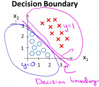
Example of a Linear Decision Boundary

Hypothesis:

$$ h_{\theta}(x) = g(\theta_0 + \theta_1x_1 + \theta_2x_2) $$

Theta Vector:

$$ \theta = \begin{bmatrix} -3 \\ 1 \\ 1 \end{bmatrix} $$

Condition for $y = 1$:

$$ -3 + x_1 + x_2 \geq 0 $$

Hence, the decision boundary is a straight line: $x_2 = -x_1 + 3$.

Here's the Python implementation:

import numpy as np
import matplotlib.pyplot as plt

# Sigmoid function
def sigmoid(z):
    return 1 / (1 + np.exp(-z))

# Hypothesis function
def hypothesis(theta, X):
    return sigmoid(np.dot(X, theta))

# Predict function
def predict(theta, X):
    return hypothesis(theta, X) >= 0.5

# Define the theta vector
theta = np.array([-3, 1, 1])

# Define the range for x1 and compute the corresponding x2 for the decision boundary
x1_vals = np.linspace(0, 5, 100)
x2_vals = -x1_vals + 3

# Plotting the decision boundary
plt.plot(x1_vals, x2_vals, label=r'$x_2 = -x_1 + 3$')
plt.xlim(0, 5)
plt.ylim(0, 5)
plt.xlabel(r'$x_1$')
plt.ylabel(r'$x_2$')
plt.title('Linear Decision Boundary')
plt.legend()
plt.grid(True)
plt.show()

Non-linear Decision Boundaries

• Purpose: To fit more complex, non-linear datasets.
• Approach: Introduce polynomial terms in the hypothesis.

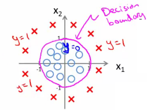
Example of a Non-linear Decision Boundary

Hypothesis:

$$ h_{\theta}(x) = g(\theta_0 + \theta_1x_1 + \theta_2x_1^2 + \theta_3x_2^2) $$

Theta Vector:

$$ \theta = \begin{bmatrix} -1 \\ 0 \\ 1 \\ 1 \end{bmatrix} $$

Condition for $y = 1$:

$$ x_1^2 + x_2^2 \geq 1 $$

This forms a circular decision boundary with radius 1 around the origin: $x_1^2 + x_2^2 = 1$.

Here's the Python implementation:

import numpy as np
import matplotlib.pyplot as plt

# Sigmoid function
def sigmoid(z):
    return 1 / (1 + np.exp(-z))

# Hypothesis function for non-linear decision boundary
def hypothesis(theta, X):
    # Compute the polynomial terms
    poly_terms = np.dot(X, theta)
    return sigmoid(poly_terms)

# Predict function
def predict(theta, X):
    return hypothesis(theta, X) >= 0.5

# Define the theta vector
theta = np.array([-1, 0, 1, 1])

# Generate a grid of values for x1 and x2
x1_vals = np.linspace(-2, 2, 400)
x2_vals = np.linspace(-2, 2, 400)
x1, x2 = np.meshgrid(x1_vals, x2_vals)

# Compute the decision boundary condition
decision_boundary = theta[0] + theta[1] * x1 + theta[2] * x1**2 + theta[3] * x2**2

# Plot the decision boundary
plt.contour(x1, x2, decision_boundary, levels=[0], linewidths=2, colors='red')
plt.xlim(-2, 2)
plt.ylim(-2, 2)
plt.xlabel(r'$x_1$')
plt.ylabel(r'$x_2$')
plt.title('Non-linear Decision Boundary')
plt.grid(True)
plt.gca().set_aspect('equal', adjustable='box')
plt.show()

Cost Function for Logistic Regression

Logistic regression uses a different cost function compared to linear regression, tailored to the classification setting.

Training Set Representation

Consider a training set of $m$ examples:

$$ {(x^{(1)}, y^{(1)}), ..., (x^{(m)}, y^{(m)})} $$

where

$$
x = \begin{bmatrix} x_0 \\ x_1 \\ ... \\ x_n \end{bmatrix} $$

with $x_0 = 1$ and $y$ being either 0 or 1.

Linear Regression Cost Function

In linear regression, the cost function $J(\theta)$ is defined as:

$$ J(\theta) = \frac{1}{2m} \sum_{i=1}^{m}(h_{\theta}(x^{(i)}) - y^{(i)})^2 $$

Defining Cost for Logistic Regression

For logistic regression, we define a different "cost" function:

$$ cost(h_{\theta}(x^{(i)}), y^{(i)}) = \frac{1}{2} (h_{\theta}(x^{(i)}) - y^{(i)})^2 $$

Redefining $J(\theta)$:

$$ J(\theta) = \frac{1}{m} \sum_{i=1}^{m}cost(h_{\theta}(x^{(i)}), y^{(i)}) $$

This cost function for logistic regression is not convex, leading to potential issues with local optima.

Logistic Regression Cost Function

The logistic regression cost function is defined as:

$$ cost(h_{\theta}(x), y) = \begin{cases} -\log(h_{\theta}(x)) & \text{if } y=1 \\ -\log(1 - h_{\theta}(x)) & \text{if } y=0 \end{cases} $$

Then, the overall cost function $J(\theta)$ becomes:

$$J(\theta) = \frac{1}{m} \sum_{i=1}^{m}[-y^{(i)}\log(h_{\theta}(x^{(i)})) - (1-y^{(i)})\log(1 - h_{\theta}(x^{(i)}))] $$

Gradient of the Cost Function

The gradient of $J(\theta)$ for logistic regression is:

$$ \frac{\partial}{\partial \theta_j} J(\theta) = \frac{1}{m} \sum_{i=1}^{m} (h_{\theta}(x^{(i)}) - y^{(i)})x_j^{(i)} $$

Note: While this gradient looks identical to that of linear regression, the formulae differ due to the different definitions of $h_{\theta}(x)$ in linear and logistic regression.

Here's the Python implementation:

import numpy as np

# Sigmoid function
def sigmoid(z):
    return 1 / (1 + np.exp(-z))

# Hypothesis function
def hypothesis(theta, X):
    return sigmoid(np.dot(X, theta))

# Cost function for logistic regression
def compute_cost(theta, X, y):
    m = len(y)
    h = hypothesis(theta, X)
    cost = (-1 / m) * np.sum(y * np.log(h) + (1 - y) * np.log(1 - h))
    return cost

# Gradient of the cost function
def compute_gradient(theta, X, y):
    m = len(y)
    h = hypothesis(theta, X)
    gradient = (1 / m) * np.dot(X.T, (h - y))
    return gradient

# Example usage
if __name__ == "__main__":
    # Sample data (X should include the intercept term)
    X = np.array([[1, 0.5, 1.5],
                  [1, 1.5, 0.5],
                  [1, 3, 3.5],
                  [1, 2, 2.5]])
    y = np.array([0, 0, 1, 1])
    
    # Initial theta
    theta = np.array([0, 0, 0])
    
    # Compute cost and gradient
    cost = compute_cost(theta, X, y)
    gradient = compute_gradient(theta, X, y)
    
    print("Cost:", cost)
    print("Gradient:", gradient)

In the example usage, we define a small sample dataset with features $X$ and labels $y$, initialize the theta vector, and compute both the cost and the gradient. The computed cost and gradient are printed out for inspection.

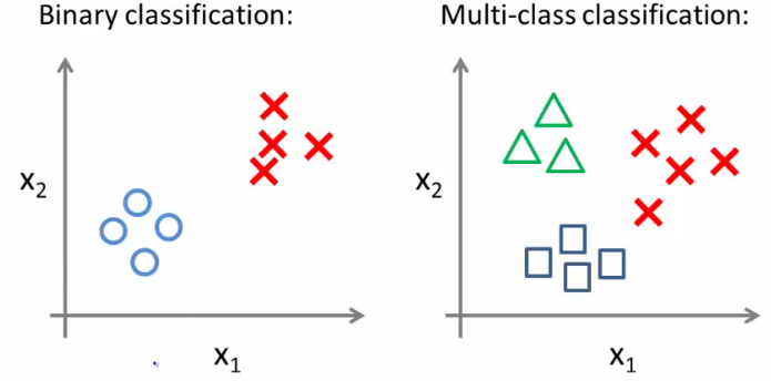
Multiclass Classification Problems

Logistic regression can be extended to handle multiclass classification problems through the "one-vs-all" (or "one-vs-rest") method.

One-vs-All Approach

The one-vs-all strategy involves training multiple binary classifiers, each focused on distinguishing one class from all other classes.

Visualization of Multiclass Classification

Consider a dataset with three classes: triangles, crosses, and squares.

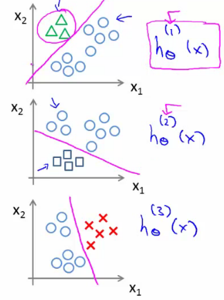
Implementing One-vs-All

The process involves splitting the training set into separate binary classification problems:

1. Triangle vs Others: Train a classifier $h_{\theta}^{(1)}(x)$ to distinguish triangles (1) from crosses and squares (0).
2. Crosses vs Others: Train another classifier $h_{\theta}^{(2)}(x)$ to distinguish crosses (1) from triangles and squares (0).
3. Squares vs Others: Lastly, train a classifier $h_{\theta}^{(3)}(x)$ to distinguish squares (1) from crosses and triangles (0).

To implement the One-vs-All (OvA) approach for multi-class classification, we need to train separate binary classifiers for each class, treating each class as the positive class and all others as the negative class. Here is the step-by-step implementation:

import numpy as np
from scipy.optimize import minimize

# Sigmoid function
def sigmoid(z):
    return 1 / (1 + np.exp(-z))

# Hypothesis function
def hypothesis(theta, X):
    return sigmoid(np.dot(X, theta))

# Cost function for logistic regression
def compute_cost(theta, X, y):
    m = len(y)
    h = hypothesis(theta, X)
    cost = (-1 / m) * np.sum(y * np.log(h) + (1 - y) * np.log(1 - h))
    return cost

# Gradient of the cost function
def compute_gradient(theta, X, y):
    m = len(y)
    h = hypothesis(theta, X)
    gradient = (1 / m) * np.dot(X.T, (h - y))
    return gradient

# One-vs-All training function
def one_vs_all(X, y, num_labels, lambda_=0.1):
    m, n = X.shape
    all_theta = np.zeros((num_labels, n + 1))
    
    # Add intercept term to X
    X = np.hstack((np.ones((m, 1)), X))
    
    # Train each classifier
    for c in range(num_labels):
        initial_theta = np.zeros(n + 1)
        options = {'maxiter': 50}
        result = minimize(compute_cost, initial_theta, args=(X, (y == c).astype(int)), method='TNC', jac=compute_gradient, options=options)
        all_theta[c] = result.x
    
    return all_theta

# Prediction function for One-vs-All
def predict_one_vs_all(all_theta, X):
    m = X.shape[0]
    X = np.hstack((np.ones((m, 1)), X))
    predictions = hypothesis(all_theta.T, X)
    return np.argmax(predictions, axis=1)

# Example usage
if __name__ == "__main__":
    # Sample data (X should include the intercept term)
    X = np.array([[0.5, 1.5],
                  [1.5, 0.5],
                  [3, 3.5],
                  [2, 2.5],
                  [1, 1],
                  [3.5, 4],
                  [2.5, 3],
                  [1, 0.5]])
    y = np.array([0, 0, 1, 1, 2, 2, 1, 0])  # 0: Triangle, 1: Cross, 2: Square
    
    # Train One-vs-All classifiers
    num_labels = 3
    all_theta = one_vs_all(X, y, num_labels)
    
    # Make predictions
    predictions = predict_one_vs_all(all_theta, X)
    print("Predictions:", predictions)
    print("Actual labels:", y)

1. We define a small sample dataset with features $X$ and labels $y$.
2. The one_vs_all function trains the classifiers.
3. The predict_one_vs_all function makes predictions on the dataset.

Classification Decision

• When classifying a new example, compute the probability that it belongs to each class using the respective classifiers.
• The class with the highest probability is chosen as the prediction.

Reference

These notes are based on the free video lectures offered by Stanford University, led by Professor Andrew Ng. These lectures are part of the renowned Machine Learning course available on Coursera. For more information and to access the full course, visit the Coursera course page.