Forward Difference Method

The forward difference method estimates a derivative from the function value at the target point $x$ and a later point $x+h$, with $h>0$. Dividing the change in the two values by their separation gives a secant slope that approximates the tangent slope at $x$. The method is useful at the left boundary of a dataset or whenever the later sample can be evaluated or obtained.

It uses a forward neighbor, whereas a backward difference uses a preceding neighbor and a central difference uses samples on both sides. If $x$ represents time, the later observation must be available before the estimate can be reported. In numerical analysis, engineering simulations, and computational modeling, this simple stencil is often a starting point for understanding derivative accuracy and the effect of sampling resolution.

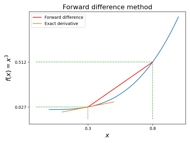
forward difference method Illustration

Mathematical formulation

The forward difference approximation of the first derivative of a function $f$ at a point $x$ with a step size $h$ is mathematically expressed as:

$$ f'(x) \approx \frac{f(x + h) - f(x)}{h} $$

This formula is derived from the fundamental definition of the derivative, which represents the instantaneous rate of change of a function at a specific point. In the context of finite differences, the forward difference method estimates this rate by calculating the difference in function values between the point $x + h$ and the point $x$, then dividing by the step size $h$. Geometrically, this approximation corresponds to the slope of the secant line that connects the points $(x, f(x))$ and $(x + h, f(x + h))$.

By focusing on the interval leading forward from $x$, the forward difference method provides an estimate of the derivative using the current sample and one later sample. It is suitable when that later value is already available, can be evaluated, or can be awaited before reporting the derivative estimate.

The simplicity of the forward difference formula allows for easy implementation in computational algorithms. However, this method introduces an approximation error, which is influenced by the choice of the step size $h$. Selecting an appropriate $h$ is crucial to balancing accuracy and numerical stability in derivative approximations.

Expanding $f(x+h)$ with Taylor's theorem gives the truncation error explicitly. For some intermediate point $\xi\in(x,x+h)$ (rather than reusing $x$ in that last term),

$$ \frac{f(x+h)-f(x)}{h} = f'(x) + \frac{h}{2}f''(\xi), $$

so the error is $\mathcal{O}(h)$: halving $h$ roughly halves the error. The method is exact for affine functions $f(x)=ax+b$ at every point and step size. For nonlinear functions the truncation error is generally nonzero, although special points or step sizes can give accidental equality.

In floating-point arithmetic the subtraction $f(x+h)-f(x)$ also contributes a roundoff error of size roughly $\varepsilon\,|f(x)|/h$, where $\varepsilon\approx 2.2\times10^{-16}$ is the machine epsilon in double precision. Balancing it against the truncation error $\frac{h}{2}|f''|$ gives an optimal step of order $h\sim\sqrt{\varepsilon}\approx 10^{-8}$ (scaled by $\sqrt{|f|/|f''|}$), with a best attainable error of about $\sqrt{\varepsilon}\approx 10^{-8}$. Choosing a much smaller $h$ makes the result worse, not better.

Derivation and step-size selection

For $f\in C^2([x,x+h])$ and $h>0$, write

$$ f(x+h)=f(x)+hf'(x)+\frac{h^2}{2}f''(\xi),\qquad \xi\in(x,x+h). $$

Subtracting $f(x)$ and dividing by $h$ gives the forward difference and its signed error. If $|f''|\leq M_2$ on this interval, the truncation error is at most $M_2h/2$. For $f(x)=x^2$, the quotient is $2x+h$, which explains the $+0.01$ error in the worked example.

A simple total-error model is

$$ E(h)\lesssim\frac{M_2}{2}h+\frac{2\delta}{h}, $$

where $\delta$ bounds the absolute error in each function evaluation. Minimizing the right-hand side gives $h_{\mathrm{opt}}\approx2\sqrt{\delta/M_2}$ when $M_2>0$. Taking $\delta$ proportional to machine precision times the function scale recovers the square-root rule. The numerical values $10^{-8}$ for step size and attainable error are scale estimates, not universal absolute guarantees.

At a left boundary, a second-order alternative using three forward samples is

$$ f'(x)\approx\frac{-3f(x)+4f(x+h)-f(x+2h)}{2h}. $$

Taylor expansion cancels the constant and second-derivative terms, leaving $f'(x)-h^2f^{(3)}(x)/3+O(h^3)$. This remains a one-sided method, so it can be used when values to the left of $x$ are unavailable. In streaming data, a forward estimate at the current time requires waiting for the later sample.

Example

Consider the function $f(x) = x^2$. We aim to approximate the derivative of this function at the point $x = 2$ using the forward difference method with a step size $h = 0.01$. Applying the forward difference formula, we perform the following calculation:

$$ f'(2) \approx \frac{f(2 + 0.01) - f(2)}{0.01} = \frac{4.0401 - 4}{0.01} = 4.01 $$

In this example, the exact derivative of $f(x) = x^2$ at $x = 2$ is $f'(2) = 2 \times 2 = 4$. The approximation obtained using the forward difference method is $4.01$, which is remarkably close to the exact value. This demonstrates the method's effectiveness in providing accurate derivative estimates, especially when the function is smooth and the step size $h$ is appropriately chosen. The accuracy of the approximation can vary depending on the function's behavior and the selected step size. For functions with rapid changes or higher curvature, smaller step sizes may be necessary to achieve comparable accuracy, albeit at the cost of increased computational effort and potential numerical instability.

Advantages

The ease of implementation and understanding allows for straightforward application of the forward difference method, which uses basic arithmetic operations, making it accessible to those with a foundational understanding of calculus and numerical methods.
Minimal data requirements ensure that the method only needs function values at $x$ and $x + h$, making it practical for discrete datasets where future function values are accessible.
The method is naturally suited to forward-progressing systems, such as time-series analysis and signal processing, where data flows sequentially, enabling efficient derivative estimation without requiring additional storage for past data.

Limitations

Approximation error is inherent in the method. Although reducing the step size $h$ improves accuracy, making $h$ too small can cause numerical instability and amplify roundoff errors, requiring a balance to maintain stability and minimize error.
Lower accuracy compared to the central difference method results from its error being of order $O(h)$, whereas the central difference method achieves $O(h^2)$ accuracy. This makes the forward difference method less precise for the same step size.
The inapplicability at domain endpoints arises from its need for function values at $x + h$, which may fall outside the defined interval at the domain's end. This requires alternative methods, such as one-sided differences, for boundary point computations.
Sensitivity to function behavior limits its reliability when the function is not smooth over the interval $[x, x + h]$, as rapid changes, discontinuities, or non-differentiable points can compromise the approximation's validity.