QR Method

The QR method computes the eigenvalues of a square matrix through a sequence of similarity transformations. Each iteration factors the current matrix into an orthogonal factor $Q$ and an upper-triangular factor $R$, then forms the product in the opposite order. The new matrix has the same eigenvalues but a different arrangement of its entries. Suitable shifts and deflation guide this process toward triangular or real block-triangular Schur form. Real eigenvalues then appear in single diagonal entries, while complex conjugate pairs are recovered from $2\times2$ diagonal blocks. The method avoids the potentially ill-conditioned task of forming a characteristic polynomial and finding all of its roots numerically.

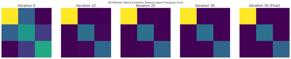
Mathematical formulation

Consider an $n \times n$ matrix $A$. The QR decomposition (factorization) of $A$ is given by:

$$ A = QR $$

where $Q$ is an orthogonal matrix ($Q^T Q = I$) and $R$ is an upper-triangular matrix.

The QR method applies the following iterative scheme:

I. Initialization: Set $A_0 = A$.

II. Iteration: For each iteration $k \geq 1$:

Compute the QR factorization of $A_{k-1}$:

$$ A_{k-1} = Q_k R_k. $$

Form a new matrix:

$$ A_k = R_k Q_k. $$

Notice that:

$$ A_k = R_k Q_k = Q_k^{-1} A_{k-1} Q_k, $$ which means $A_k$ is similar to $A_{k-1}$. Since similarity transformations preserve eigenvalues, all $A_k$ share the same eigenvalues as the original matrix $A$.

As $k$ increases, under certain conditions (e.g., when shifts such as the Wilkinson shift are used), the matrix $A_k$ converges to an upper-triangular matrix (or a quasi-upper-triangular form in the real case), whose diagonal entries give real eigenvalues in the triangular case. In real quasi-triangular form, each $2\times2$ diagonal block must instead be solved for its conjugate-pair eigenvalues.

Derivation

The idea behind the QR method arises from the following observations:

Step 1: Similarity and eigenvalues.

Two matrices $A$ and $B$ are similar if there exists an invertible matrix $C$ such that $A = C^{-1} B C$. Similar matrices share the same eigenvalues.

Step 2: QR decomposition.

Every real square matrix $A$ can be decomposed into an orthogonal matrix $Q$ and an upper-triangular matrix $R$ (the factorization is unique if $A$ is invertible and $R$ is required to have a positive diagonal).

Step 3: Iterative process.

By repeatedly factoring $A_{k-1}$ into $Q_k R_k$ and then forming $A_k = R_k Q_k$, we create a sequence of similar matrices $A_0, A_1, A_2, \ldots$. If $A_k$ converges to an upper-triangular matrix, the eigenvalues are the diagonal elements of that limit.

In practice, shifts are employed to speed up convergence (the so-called "QR algorithm with shifts"). Each step factors $A_{k-1} - \mu_k I = Q_k R_k$ and forms $A_k = R_k Q_k + \mu_k I$, which is still similar to $A_{k-1}$. A standard choice is the Wilkinson shift: $\mu_k$ is the eigenvalue of the trailing $2 \times 2$ block of $A_{k-1}$ that is closest to its bottom-right entry $a_{nn}$.

For a real matrix whose trailing block has a complex conjugate pair, no real shift equals an eigenvalue of that block, so both conjugate shifts are applied together in one real step (a double shift). With suitable shifts, the subdiagonal coupling to the trailing block can become small rapidly, allowing that eigenvalue or conjugate pair to be deflated. Local rates can be quadratic or, for generic symmetric cases, cubic; these rates depend on the matrix and shift and are not universal guarantees. The diagonal eigenvalue itself does not converge to zero.

Schur form and the role of orthogonal transformations

After $k$ unshifted steps, let $Z_k=Q_1Q_2\cdots Q_k$. Repeated substitution gives $A_k=Z_k^\top AZ_k$. Each factor is orthogonal, so the cumulative change of basis preserves Euclidean norms rather than amplifying errors through an arbitrary inverse.

The real endpoint is the real Schur form, whose diagonal blocks have size one or two. For a block $B=\begin{bmatrix}a&b\\c&d\end{bmatrix}$, its two eigenvalues solve $\lambda^2-(a+d)\lambda+ad-bc=0$. A conjugate pair is represented by such a block even though the original matrix and the arithmetic are real.

Practical implementations first reduce $A$ to upper Hessenberg form, with zeros below the first subdiagonal. They then preserve that structure during shifted iterations and deflate small couplings using scale-aware tolerances. Householder transformations or Givens rotations provide more reliable orthogonality than classical Gram–Schmidt in finite precision. The LAPACK Users' Guide describes this distinction between eigenvectors and Schur vectors.

Algorithm steps

Step 1: Initialization. Set $A_0 = A$.

Step 2: QR factorization. Compute the QR factorization of $A_{k-1}$:

$$ A_{k-1} = Q_k R_k. $$

The QR factorization can be computed using:

• Gram-Schmidt orthogonalization,
• Householder transformations,
• or Givens rotations.

Step 3: Form new matrix.

$$ A_k = R_k Q_k. $$

Note that:

$$ A_k = Q_k^{-1} A_{k-1} Q_k, $$

so $A_k$ and $A_{k-1}$ are similar.

Step 4: Check for convergence.

For a real matrix, test whether the required subdiagonal couplings are small enough to isolate $1\times1$ or $2\times2$ diagonal blocks. Entries above the diagonal generally remain nonzero. A real complex-pair block must not be forced to become diagonal.

Step 5: Output.

Read the eigenvalues from the $1\times1$ and $2\times2$ diagonal blocks of the real Schur form. In the complex triangular form, all eigenvalues appear directly on the diagonal.

Example

Given System:

$$ A = \begin{bmatrix}4 & 1 \\ 2 & 3\end{bmatrix}. $$

Step 1: First QR factorization.

Perform the QR factorization on $A_0 = A$.

Suppose we find:

$$ A = Q_1 R_1, $$ with

$$ Q_1 = \begin{bmatrix}0.8944 & -0.4472 \\ 0.4472 & 0.8944\end{bmatrix}, \quad R_1 = \begin{bmatrix}4.4721 & 2.2361 \\ 0 & 2.2361\end{bmatrix}. $$

Step 2: Form $A_1$.

$$ A_1 = R_1 Q_1. $$

Using exact forms $Q_1=\frac1{\sqrt5}\begin{bmatrix}2&-1\\1&2\end{bmatrix}$ and $R_1=\begin{bmatrix}2\sqrt5&\sqrt5\\0&\sqrt5\end{bmatrix}$ gives

$$ A_1=\begin{bmatrix}5&0\\1&2\end{bmatrix}. $$

The trace remains $7$ and the determinant remains $10$, as similarity requires. These checks help distinguish rounding in the displayed factors from an incorrect transformation.

After multiplication, ideally, we move closer to an upper-triangular form. Repeating this process multiple times (depending on the complexity of the matrix) will reduce the entries below the eventual triangular or block-triangular structure; the entries above the diagonal need not approach zero.

Step 3: Convergence.

After sufficient iterations, the matrix $A_k$ will approximate an upper-triangular matrix. The diagonal entries of this matrix give the eigenvalues of $A$.

For this simple $2 \times 2$ matrix, the method would quickly converge. The eigenvalues obtained would match the exact eigenvalues solved by the characteristic equation.

Advantages

I. All Eigenvalues Simultaneously:

The QR method retrieves all eigenvalues of a matrix at once, rather than computing them individually.

II. Numerical Stability:

Orthogonal transformations preserve Euclidean lengths, and shifted QR with deflation is a standard basis for dense eigenvalue solvers. A stable implementation controls rounding while working directly with the matrix, rather than introducing the additional sensitivity of a characteristic-polynomial calculation. The Hessenberg reduction and Schur-form discussion above explain the structure used by those solvers.

III. Broad Applicability:

The QR method works for both real and complex matrices and can be adapted to handle a variety of matrix types efficiently.

Limitations

I. No Direct Eigenvectors:

The basic QR algorithm finds eigenvalues but does not directly produce eigenvectors. Additional steps or modifications are required to recover eigenvectors.

II. Computational Effort:

Although efficient algorithms exist, the QR method can be computationally intensive for very large matrices. Advanced techniques like the Hessenberg form and modern parallel algorithms are used to improve performance.

III. Convergence Speed for Certain Matrices:

While generally fast, convergence can be slow if the matrix has certain structures or if shifts are not chosen wisely, making it less practical without proper optimization.

For a dense $n \times n$ matrix, one unshifted QR step costs $O(n^3)$. After a one-time reduction to Hessenberg form ($O(n^3)$), each step costs only $O(n^2)$, and with shifts and deflation the whole eigenvalue computation takes $O(n^3)$ operations.