Trapezoidal Rule

The trapezoidal rule approximates a definite integral by connecting neighboring samples with straight line segments and integrating those segments. When the sampled values are nonnegative, each contribution is the area of a trapezoid; negative values contribute signed area in the same way as the exact integral. The method is useful in engineering, physics, economics, and other settings where an antiderivative is unavailable or the function is known only through data.

Dividing the interval into smaller pieces lets the line segments follow changes in the curve. Compared with using only the left or right endpoint for each rectangle, averaging both endpoints cancels the leading slope contribution to the composite error. Its simplicity and predictable cost make it useful both for direct calculations and as a basis for extrapolation methods.

Mathematical formulation

The mathematical foundation of the trapezoidal rule is based on the assumption that the region under the graph of a function $f(x)$ over a given interval $[a, b]$ can be approximated by a trapezoid. A trapezoid is a quadrilateral with at least one pair of parallel sides, which in this context are the vertical segments at $x = a$ and $x = b$ of lengths $f(a)$ and $f(b)$, while the top side is the line connecting the points $(a, f(a))$ and $(b, f(b))$. The area of this trapezoid provides an estimate of the definite integral of the function over the interval $[a, b]$.

The basic formula for the trapezoidal rule when applied to a single interval $[a, b]$ is:

$$ \frac{b - a}{2} [f(a) + f(b)] $$

This formula calculates the area of the trapezoid by taking the average of the function values at the endpoints $f(a)$ and $f(b)$, and then multiplying by the width of the interval $(b - a)$. This approximation assumes that the function behaves linearly between the two endpoints, which is a reasonable assumption for small intervals or functions that do not vary drastically.

To improve the accuracy of the approximation, the interval $[a, b]$ can be divided into $n$ smaller subintervals of equal width. Let $h$ represent the width of each subinterval, calculated as:

$$ h = \frac{b - a}{n} $$

Within each subinterval $[x_i, x_{i+1}]$, the function $f(x)$ is evaluated at the endpoints $x_i$ and $x_{i+1}$. The area of each trapezoid within these subintervals is then computed using the formula:

$$ \frac{f(x_{i+1}) + f(x_i)}{2} h $$

The integral $I$ over the entire interval $[a, b]$ is then approximated by summing the areas of all the trapezoids:

$$ T_n = \sum_{i=0}^{n-1} \frac{f(x_{i+1}) + f(x_i)}{2} h $$

This summation effectively aggregates the contributions of each trapezoid to estimate the total area under the curve $f(x)$ across the interval. The graphical representation below illustrates how the trapezoidal rule approximates the area under a curve by stacking trapezoids side by side:

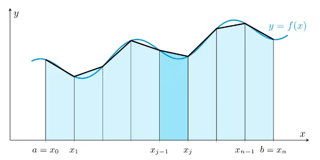
In this diagram, each trapezoid corresponds to a subinterval $[x_i, x_{i+1}]$, with the parallel sides representing the function values $f(x_i)$ and $f(x_{i+1})$. The height of each trapezoid is the width $h$ of the subinterval, and the area of each trapezoid contributes to the overall approximation of the integral.

Error term

For a twice continuously differentiable $f$, the composite trapezoidal rule with $n$ subintervals of width $h = \frac{b-a}{n}$ satisfies

$$ \int_a^b f(x)\,dx - T_n = -\frac{b-a}{12} h^2 f''(\xi), \qquad \xi \in (a, b). $$

The rule is exact for polynomials of degree one or lower and is second-order accurate, $O(h^2)$. For convex functions ($f'' > 0$) it overestimates the integral.

Integrating the linear interpolant

On one panel $[u,v]$ of width $h=v-u$, the line through the endpoint samples is

$$ p(x)=f(u)\frac{v-x}{h}+f(v)\frac{x-u}{h}. $$

Both basis functions integrate to $h/2$, producing $h[f(u)+f(v)]/2$. For $f\in C^2$, the interpolation remainder is $f(x)-p(x)=f''(\xi_x)(x-u)(x-v)/2$. Since the polynomial weight has one sign on the panel, integration and the weighted mean value theorem give

$$ \int_u^v(f(x)-p(x))\,dx=-\frac{h^3}{12}f''(\xi). $$

Summing panels proves the composite error formula. For $x^2$ on $[0,2]$ with $h=1$, it predicts $I-T_2=-(2/12)\cdot2=-1/3$, agreeing with $8/3-3$.

Combining repeated endpoints also gives the convenient form

$$ T_n=h\left[\frac{f(a)}2+\sum_{i=1}^{n-1}f(x_i)+\frac{f(b)}2\right]. $$

It needs $n+1$ evaluations. For unequally spaced data, use $\sum_i(x_{i+1}-x_i)[f(x_i)+f(x_{i+1})]/2$ instead of a common $h$. Negative sampled values contribute signed area, just as in the exact integral.

If a smooth uniform-grid error expansion applies, $(4T_{2n}-T_n)/3$ cancels the leading $h^2$ error. This is Simpson's rule on the refined grid and is the first extrapolation step behind Romberg integration. Smooth periodic functions can exhibit much faster trapezoidal convergence than the generic second-order bound suggests.

Algorithm steps

Implementing the trapezoidal rule involves a systematic process to ensure an accurate approximation of the definite integral. The following steps outline the procedure:

Step 1: Partition the interval.

• Begin by dividing the interval $[a, b]$ into $n$ equal subintervals. The number of subintervals $n$ determines the granularity of the approximation; a larger $n$ generally leads to a more accurate result.
• Calculate the width of each subinterval using the formula:

$$ h = \frac{b - a}{n} $$

This step ensures that the interval is evenly partitioned, facilitating consistent application of the trapezoidal rule across all subintervals.

Step 2: Evaluate function at endpoints.

• For each subinterval $[x_i, x_{i+1}]$, compute the function values at the endpoints $f(x_i)$ and $f(x_{i+1})$.
• These evaluations are crucial as they determine the heights of the trapezoids that approximate the area under the curve within each subinterval.
• Organizing these function values systematically allows for efficient computation of the trapezoidal areas.

Step 3: Apply the trapezoidal rule formula.

• Use the trapezoidal rule formula to calculate the area of each trapezoid within the subintervals:

$$ \frac{f(x_{i+1}) + f(x_i)}{2} h $$

• This formula takes the average of the function values at the endpoints and multiplies it by the width $h$ to determine the area of the trapezoid.
• Applying this formula uniformly across all subintervals ensures consistency and accuracy in the approximation process.

Step 4: Aggregate the results.

Sum the areas of all the trapezoids computed in the previous step to obtain the total integral approximation:

$$ T_n = \sum_{i=0}^{n-1} \frac{f(x_{i+1}) + f(x_i)}{2} h $$

• This aggregation provides the final estimate of the definite integral over the interval $[a, b]$.
• The sum effectively captures the cumulative area under the curve as approximated by the series of trapezoids.

The resulting sum is the exact integral of the piecewise linear curve through the sampled points. Shared interior endpoints receive contributions from two neighboring panels, while each outer endpoint contributes to one panel. Once the values are available, evaluation needs only a weighted sum, with work proportional to the number of panels. Its accuracy is then governed by the sampling and curvature estimates discussed above, making the cost and error sources explicit.

Example

To illustrate the application of the trapezoidal rule, consider the function $f(x) = x^2$. This example demonstrates how the method approximates the integral over a specific interval using a manageable number of subintervals.

Step 1: Choose interval and subdivisions.

• Let $a = 0$ and $b = 2$, and partition this interval into $n = 2$ equal subintervals. This choice ensures that the interval is evenly divided, facilitating the application of the trapezoidal rule.
• Calculate the width of each subinterval:

$$ h = \frac{2 - 0}{2} = 1 $$

This results in two subintervals: $[0, 1]$ and $[1, 2]$, each with a width of 1.

Step 2: Evaluate function at endpoints.

Compute the function values at the endpoints of each subinterval:

For the first subinterval $[0, 1]$:

• $f(0) = 0^2 = 0$
• $f(1) = 1^2 = 1$

For the second subinterval $[1, 2]$:

• $f(1) = 1^2 = 1$
• $f(2) = 2^2 = 4$

These evaluations provide the necessary data points for calculating the areas of the trapezoids.

Step 3: Apply the trapezoidal rule formula.

Calculate the area of each trapezoid using the trapezoidal rule formula:

For $[0, 1]$:

$$ \frac{1 - 0}{2} [f(0) + f(1)] = \frac{1}{2} (0 + 1) = 0.5 $$

For $[1, 2]$:

$$ \frac{2 - 1}{2} [f(1) + f(2)] = \frac{1}{2} (1 + 4) = 2.5 $$

These calculations yield the areas of the trapezoids corresponding to each subinterval.

Step 4: Sum the areas.

Add the areas of the individual trapezoids to obtain the total integral approximation:

$$ T_2 = 0.5 + 2.5 = 3 $$

This sum represents the estimated value of the definite integral of $f(x) = x^2$ over the interval $[0, 2]$ using the trapezoidal rule.

Step 5: Compare with exact integral.

For validation, compute the exact value of the integral analytically:

$$ \int_{0}^{2} x^2 \, dx = \left[\frac{x^3}{3} \right]_0^2 = \frac{8}{3} \approx 2.6667 $$

The trapezoidal rule approximation of 3 is reasonably close to the exact value of approximately 2.6667, demonstrating the method's effectiveness even with a small number of subintervals.

This example highlights the practical application of the trapezoidal rule and illustrates how it provides a balance between computational simplicity and accuracy. While the approximation is not exact in this case, it is sufficiently close for many practical purposes, especially when dealing with functions that do not exhibit extreme behavior within the interval of integration.

Advantages

• The trapezoidal rule is straightforward to understand and implement, making it accessible to students and practitioners alike. The method relies on basic arithmetic operations and function evaluations at specific points, without requiring complex algorithms or iterative procedures.
• Compared to the Rectangle Rule, which approximates the area under a curve using rectangles based on function values at the left or right endpoints, the trapezoidal rule often provides a more accurate approximation (the midpoint rule has half the standard second-derivative error-bound constant on the same partition, although actual errors need not have this ratio). This increased accuracy stems from the method's ability to account for the linear trend between two consecutive points, effectively averaging the function's behavior over each subinterval.
• The trapezoidal rule is versatile and can be applied to a broad spectrum of functions, including those that are linear, polynomial, or exhibit smooth curvature. It is particularly effective for functions that do not have extreme fluctuations or sharp bends within the interval of integration.
• The method is computationally efficient, especially for functions that are computationally inexpensive to evaluate. Since the composite trapezoidal rule requires only one new function evaluation per subinterval (adjacent subintervals share endpoints), it scales well with increasing numbers of subintervals, maintaining reasonable computational demands even for large-scale problems.
• The trapezoidal rule serves as a foundational technique in numerical integration, providing a basis for more advanced methods such as Simpson's rule and Gaussian Quadrature. Understanding the principles of the trapezoidal rule facilitates the comprehension and implementation of these more sophisticated techniques.

Limitations

• The trapezoidal rule assumes that the function behaves linearly within each subinterval, which can lead to significant approximation errors for functions that exhibit high curvature or rapid changes within the interval of integration. In such cases, the linear approximation may not capture the function's true behavior, resulting in overestimation or underestimation of the area under the curve.
• Achieving a high level of precision with the trapezoidal rule often requires dividing the interval $[a, b]$ into a large number of subintervals. While increasing the number of subintervals can enhance the accuracy of the approximation, it also increases the computational effort, as more function evaluations and calculations are necessary.
• The accuracy of the trapezoidal rule is highly dependent on the behavior of the function being integrated. For functions that are not smooth or that have irregular behavior within the interval, the linear approximations used by the trapezoidal rule may not adequately capture the true nature of the function.
• When dealing with a large number of subintervals, especially in computational implementations, the trapezoidal rule can be susceptible to the accumulation of numerical errors. These errors may arise from factors such as roundoff errors in floating-point arithmetic or from inaccuracies in function evaluations.
• The trapezoidal rule is primarily designed for definite integrals over finite intervals. It is not inherently suited for improper integrals, where the interval of integration is infinite or where the integrand has singularities within the interval.
• The standard second-order error bound assumes a continuous second derivative. For bounded piecewise continuous functions, the rule can still converge, but jumps or corners may reduce the convergence rate and invalidate that bound. Splitting the integral at known nonsmooth points makes the approximation easier to control; singularities require separate treatment.