Linear Interpolation

Linear interpolation estimates a value between two known points by assuming the function is a straight line over that interval.

Given two points

$$ (x_0,y_0), \qquad (x_1,y_1), $$

with $x_0\ne x_1$, the interpolated value at a query $x$ is

$$ L(x) = y_0 + \frac{x-x_0}{x_1-x_0}(y_1 - y_0). $$

A particularly useful form introduces the normalized coordinate

$$ t = \frac{x-x_0}{x_1-x_0}. $$

Then

$$ L(x) = (1 - t)y_0 + t y_1. $$

When $x$ lies between the endpoints, $0\le t\le1$, so the result is a weighted average of the endpoint values.

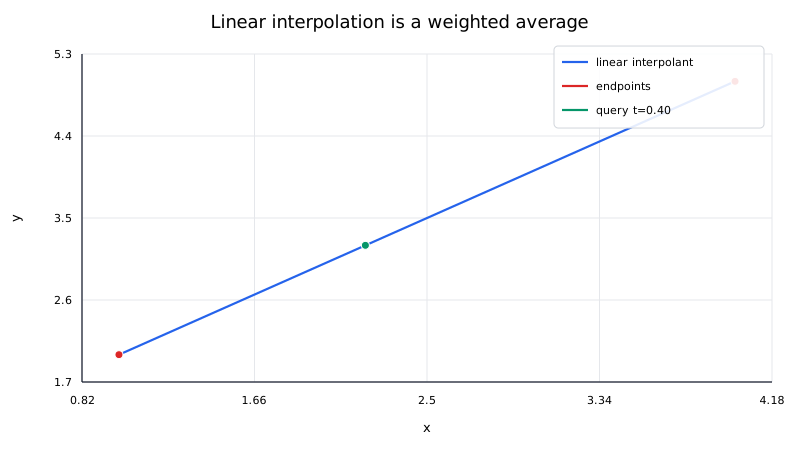
Geometric interpretation

The slope between the two samples is

$$ m = \frac{y_1-y_0}{x_1-x_0}. $$

The line through $(x_0,y_0)$ is therefore

$$ L(x) = y_0 + m(x - x_0). $$

This formula is exactly the same as the weighted form above.

The weights

$$ 1 - t \quad \text{and}\quad t $$

sum to one. That has an important consequence: if $x$ is between $x_0$ and $x_1$, then $L(x)$ lies between $y_0$ and $y_1$. A single linear segment cannot overshoot its two endpoint values.

Worked example

Take

$$ (x_0,y_0) = (1,2), \qquad (x_1,y_1) = (4,5), $$

and estimate the value at

$$ x = 2.2. $$

First compute the normalized position:

$$ t = \frac{2.2-1}{4-1} = \frac{1.2}{3} = 0.4. $$

Then

$$ L(2.2) = (1 - 0.4)\cdot2 + 0.4\cdot5 = 1.2 + 2 = 3.2. $$

So

$$ \boxed{L(2.2)=3.2}. $$

The calculation can also be read geometrically: the query is $40\%$ of the way from $x_0$ to $x_1$, so its interpolated value is $40\%$ of the way from $y_0$ to $y_1$.

Piecewise linear interpolation

For many ordered data points

$$ x_0<x_1<\cdots<x_n, $$

piecewise linear interpolation applies the same two-point formula on each interval.

If

$$ x_i\le x\le x_{i+1}, $$

then

$$ L_i(x) = y_i + \frac{x-x_i}{x_{i+1}-x_i} (y_{i+1} - y_i). $$

The resulting interpolant is continuous because adjacent segments meet at the shared data points.

However, its derivative is generally discontinuous. On interval $[x_i,x_{i+1}]$,

$$ L_i'(x) = \frac{y_{i+1}-y_i}{x_{i+1}-x_i}, $$

which is constant on that interval. At an interior node, the slope usually jumps from one secant slope to the next.

Why grid refinement helps

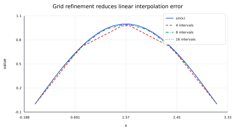
For a smooth function, shorter intervals usually make the straight-line approximation more accurate.

If $f$ is twice continuously differentiable on $[x_i,x_{i+1}]$, the interpolation error satisfies

$$ f(x) - L_i(x) = \frac{f''(\xi_x)}{2} (x - x_i)(x - x_{i+1}) $$

for some $\xi_x$ in the interval.

Let

$$ h_i = x_{i+1} - x_i. $$

The product

$$ |(x - x_i)(x - x_{i+1})| $$

is largest at the midpoint and equals $h_i^2/4$ there. Therefore,

$$ |f(x) - L_i(x)| \le \frac{h_i^2}{8} \max_{\xi\in[x_i,x_{i+1}]} |f''(\xi)|. $$

This explains the familiar second-order behavior: if the maximum interval width is reduced by roughly a factor of two, the interpolation error for a smooth function often decreases by roughly a factor of four.

Algorithm

For a single query in sorted data:

I. verify that the query lies in the permitted range;

II. locate the interval $[x_i,x_{i+1}]$ containing the query;

III. compute

$$ t = \frac{x-x_i}{x_{i+1}-x_i}; $$

IV. return

$$ (1 - t)y_i + t y_{i+1}. $$

A binary search locates the interval in $O(\log n)$ time. The interpolation itself is constant-time work.

For many sorted queries, a single pass through the nodes and queries can avoid repeating binary searches.

Numerical details

The formula

$$ y_i + t(y_{i+1} - y_i) $$

is often preferable in code to separately constructing a slope and intercept. It works directly with the local interval and keeps the calculation compact.

Important checks include:

• reject duplicate nodes because $x_{i+1}-x_i=0$ would cause division by zero;
• decide how to handle a query exactly equal to a node;
• decide whether to clamp, reject, or extrapolate out-of-range queries;
• use a data type with sufficient precision for the scale of the coordinates.

When $x_i$ and $x_{i+1}$ are extremely large but very close together relative to machine precision, the difference $x_{i+1}-x_i$ can lose relative accuracy. Rescaling or shifting the coordinate system can help.

Extrapolation

If $x$ lies outside $[x_i,x_{i+1}]$, the same formula still produces a number, but then either

$$ t<0 \qquad \text{or} \qquad t>1. $$

The weights are no longer both between zero and one, and the result is linear extrapolation rather than interpolation.

Extrapolation can be reasonable over a short distance when a linear trend is justified, but it should not be treated as automatically reliable.

Advantages

Linear interpolation is attractive because it is:

• simple to derive and implement;
• local;
• inexpensive;
• exact at the nodes;
• free from overshoot inside each interval;
• easy to update when new nodes are added.

Limitations

Its main limitation is smoothness. The interpolant is only piecewise linear, so corners appear at most interior nodes. If derivatives are important, a cubic spline or another smooth method may be a better choice.

Linear interpolation also ignores curvature inside an interval. A long interval over a highly curved function can produce a noticeable error even though the endpoint values are exact.