Heun's Method
Heun's method improves Euler's method by using information from both ends of each step. It is a second-order explicit Runge–Kutta method and is also known as the explicit trapezoidal method or improved Euler method.
For the IVP
$$ u'(t) = f(t,u), \qquad u(t_0) = u_0, $$
Euler uses only the slope at the beginning of a step. Heun first predicts the endpoint, evaluates the slope there, and then advances using the average of the two slopes.
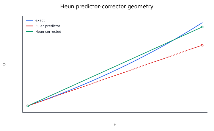
Predictor-corrector form
Given $(t_n,u_n)$ and step size $h$:
Predictor
$$ \widetilde{u}_{n+1} = u_n + h f(t_n,u_n). $$
Corrector
$$ u_{n+1} = u_n + \frac{h}{2} \left[f(t_n,u_n) + f(t_n + h,\widetilde{u}_{n+1}) \right]. $$
The predictor is an Euler step. The corrector replaces Euler's single slope by the average of the start and predicted-end slopes.
Why the average helps
The exact solution satisfies
$$ u(t_{n+1}) - u(t_n) = \int_{t_n}^{t_{n+1}} f(t,u(t))\, dt. $$
If this integral is approximated by the trapezoidal rule,
$$ u(t_{n+1}) \approx u(t_n) + \frac{h}{2} \left[f(t_n,u(t_n)) + f(t_{n+1},u(t_{n+1})) \right]. $$
The unknown endpoint $u(t_{n+1})$ would make this implicit. Heun avoids that by replacing it with the Euler prediction $\widetilde{u}_{n+1}$.
The result has:
- local truncation error: $O(h^3)$,
- global error: $O(h^2)$.
Halving $h$ therefore reduces the global error by roughly a factor of four.
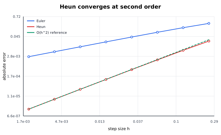
Verifying second-order accuracy
Start a step from the exact value $u=u(t_n)$ and assume the derivatives needed below are bounded. Write $f=f(t_n,u)$, and use $f_u$ for the derivative with respect to the state. Taylor expansion of the predicted-end slope gives
$$ f(t_n+h,u+hf)=f+h(f_t+f_uf)+O(h^2). $$
The corrected step is therefore
$$ u_{n+1}=u+hf+\frac{h^2}{2}(f_t+f_uf)+O(h^3). $$
Differentiating the ODE gives $u''=f_t+f_uf$, so this matches the exact Taylor expansion through $h^2$. The one-step defect is $O(h^3)$ and, under a Lipschitz error-propagation bound, the global error is $O(h^2)$. For systems, $f_u$ is the Jacobian and $f_uf$ is a matrix-vector product.
The Euler predictor differs from the true endpoint by $O(h^2)$. A Lipschitz $f$ transfers that discrepancy to an $O(h^2)$ slope error; multiplying the slope by $h$ contributes only $O(h^3)$ to the corrected state. This is why using the predictor preserves second order.
Heun performs one correction. Solving the endpoint trapezoidal equation implicitly is a different method with different stability properties. Repeating corrections would require a separate convergence argument rather than automatically turning the explicit method into an unconditionally stable solver.
Worked example
Use
$$ u' = u, \qquad u(0) = 1, $$
with $h=0.05$.
For the first step:
$$ k_1 = f(0,1) = 1, $$
$$ \widetilde{u}_1 = 1 + 0.05(1) = 1.05, $$
$$ k_2 = f(0.05,1.05) = 1.05. $$
Then
$$ u_1 = 1 + \frac{0.05}{2}(1 + 1.05) = 1.05125. $$
For the second step:
$$ \widetilde{u}_2 = 1.05125 + 0.05(1.05125) = 1.1038125, $$
and therefore
$$ u_2 = 1.05125 + \frac{0.05}{2} (1.05125 + 1.1038125) = 1.1051265625. $$
The exact value is $e^{0.1}\approx1.105170918$, so Heun is much closer than Euler with the same step size.
Runge–Kutta interpretation
Heun can be written as
$$ k_1 = f(t_n,u_n), $$
$$ k_2 = f(t_n + h,u_n + h k_1), $$
$$ u_{n+1} = u_n + \frac{h}{2}(k_1 + k_2). $$
This is a two-stage explicit Runge–Kutta method. It uses two evaluations of $f$ per step instead of one.
Distinguishing the two common second-order formulas
Heun's endpoint predictor and averaged-slope update differ from the explicit midpoint method, which evaluates a predicted midpoint and uses that slope alone:
$$ k_1=f(t_n,u_n),\qquad k_2=f(t_n+h/2,u_n+hk_1/2),\qquad u_{n+1}=u_n+hk_2. $$
Both methods have order two and the same stability polynomial on $u'=\lambda u$, but they generally produce different values on nonlinear equations. Names such as “improved Euler” can vary between references; the stage formulas identify the actual algorithm unambiguously.
Algorithm
t = t0
u = u0

while t < tf:
    h_n = min(h, tf - t)    # shorten the last step to land on tf
    k1 = f(t, u)
    predictor = u + h_n*k1
    k2 = f(t + h_n, predictor)

    u = u + h_n*(k1 + k2)/2
    t = t + h_n
Repository implementation
heun_method takes a final time t_end and a nominal step h. When (t_end - t0)/h is not an integer, the last step is shortened so that the returned grid ends exactly at t_end; all earlier steps have length h. The returned array has shape (n + 1,) for a scalar ODE (one component) and (n + 1, d) for a system with d components.
Accuracy versus cost
Compared with Euler:
| Method | Function evaluations per step | Global order |
|---|---|---|
| Euler | 1 | 1 |
| Heun | 2 | 2 |
A Heun step costs about twice as much if evaluating $f$ dominates the work, but its error decreases much faster under step refinement.
Stability
Applied to
$$ u' = \lambda u, $$
Heun produces the amplification factor
$$ R(z) = 1 + z + \frac{z^2}{2}, \qquad z = h\lambda. $$
The method is stable for values of $z$ satisfying
$$ |R(z)|\le 1. $$
On the negative real axis this is $-2\le z\le 0$, the same interval as for Euler. The region is larger than Euler's disk $|1+z|\le1$ off the real axis, but Heun is still explicit and is not a good default for strongly stiff systems.
Advantages
- Second-order accuracy with a simple formula.
- Easy to understand as a predictor-corrector method.
- More accurate than Euler for a similar conceptual complexity.
- Useful as a building block for more general Runge–Kutta schemes.
Limitations
- Requires two evaluations of $f$ per step.
- Still uses an explicit stability region.
- Fixed-step implementations do not automatically adapt to difficult portions of a trajectory.
- Stiff systems generally require implicit methods.