Midpoint Rule

The midpoint rule approximates a definite integral by dividing its interval into smaller pieces and representing each piece by a rectangle. The rectangle's width is the subinterval width, and its height is the function value at that subinterval's midpoint. Adding the signed rectangle areas estimates the total integral. This is useful when an antiderivative is unavailable or difficult to compute, but the function can be sampled inside the interval. Subdivision lets the rectangles follow changes in the function more closely. The symmetry of each midpoint panel also gives a specific accuracy benefit: the leading linear variation about the midpoint cancels when integrated.

Unique to this method, the height of each rectangle is determined by the function's value at the midpoint of the corresponding subinterval. This approach often leads to a more accurate estimate of the area than other methods like the trapezoidal rule. The midpoint value represents the entire subinterval with a single sample. Symmetry makes the linear variation about that midpoint integrate to zero, leaving curvature as the leading error source. This explains its improvement over left- or right-endpoint rectangles and the standard error-constant comparison with trapezoidal quadrature; it does not guarantee that one midpoint captures unresolved variation.

Mathematical formulation

For a function $f(x)$ defined over an interval $[a, b]$, the midpoint rule provides an approximation for the integral by evaluating the function at specific points within each subinterval. The basic formula for a single subinterval is:

$$ (b - a) f\left(\frac{a+b}{2}\right) $$

This formula calculates the area of a single rectangle whose width is the length of the interval $(b - a)$ and whose height is the function value at the midpoint $\frac{a+b}{2}$. To achieve a better approximation, the interval $[a, b]$ is divided into $n$ subintervals of equal width. The width of each subinterval, denoted by $h$, is given by:

$$ h = \frac{b - a}{n} $$

Within each subinterval, defined by $x_{i}$ and $x_{i+1}$, the function $f(x)$ is evaluated at the midpoint $\frac{x_{i} + x_{i+1}}{2}$. This gives rise to the coordinates of the rectangle:

$\left(x_{i}, f\left(\frac{x_{i} + x_{i+1}}{2}\right)\right)$
$\left(x_{i+1}, f\left(\frac{x_{i} + x_{i+1}}{2}\right)\right)$
$\left(x_{i+1}, 0\right)$
$\left(x_{i}, 0\right)$

The area of each rectangle is then computed by multiplying the height $f\left(\frac{x_{i} + x_{i+1}}{2}\right)$ by the width $h$. The integral approximation is obtained by summing these areas across all subintervals:

$$ M_n = \sum_{i=0}^{n-1} f\left(\frac{x_{i} + x_{i+1}}{2}\right) h $$

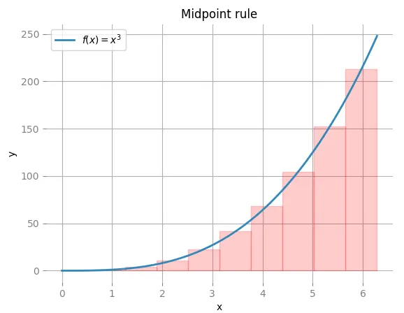
This summation provides an estimate of the total area under the curve $f(x)$ over the interval $[a, b]$. The graphical representation of this method helps visualize how the midpoint rule approximates the integral by stacking these rectangles side by side.

midpoint rule Visualization

Error term

For a twice continuously differentiable $f$, the composite midpoint rule with $n$ subintervals of width $h = \frac{b-a}{n}$ has error

$$ \int_a^b f(x)\,dx - M_n = \frac{b-a}{24} h^2 f''(\xi), \qquad \xi \in (a, b). $$

The rule is exact for polynomials of degree one or lower and is second-order accurate, $O(h^2)$. Its error constant is half that of the trapezoidal rule (which is $\frac{b-a}{12}h^2 f''(\xi)$ with the opposite sign).

Deriving the error constant

On a single panel with midpoint $m$ and width $h$, set $x=m+t$, where $-h/2\leq t\leq h/2$. Taylor expansion separates the constant, odd, and curvature terms:

$$ f(m+t)=f(m)+tf'(m)+\frac{t^2}{2}f''(\xi_t). $$

The odd term integrates to zero. The nonnegative weight $t^2/2$ and continuity of $f''$ allow a weighted mean value argument, so

$$ \int_{m-h/2}^{m+h/2}f(x)\,dx-hf(m)=f''(\xi)\int_{-h/2}^{h/2}\frac{t^2}{2}\,dt=\frac{h^3}{24}f''(\xi). $$

Summing $n$ panels changes the scale from $h^3$ locally to $nh^3=(b-a)h^2$ globally. Consequently,

$$ |I-M_n|\leq\frac{b-a}{24}h^2\max_{[a,b]}|f''|. $$

For a convex function the rule underestimates the integral; for a concave function it overestimates. In the example, $f''=2$ and $h=1$, so the error is exactly $2\cdot1^2\cdot2/24=1/6$, agreeing with $8/3-2.5$.

The midpoint error-bound constant is half the trapezoidal constant on the same uniform partition. This comparison is a bound, not a guarantee that every integrand is approximated twice as accurately: cancellation, periodicity, and the sampled locations can change the actual errors substantially.

Algorithm steps

Begin by dividing the interval $[a, b]$ into $n$ equal subintervals. The choice of $n$ determines the number of rectangles used in the approximation and affects the accuracy of the result.
For each subinterval, calculate the midpoint $\frac{x_{i} + x_{i+1}}{2}$. Evaluate the function $f(x)$ at this midpoint to determine the height of the corresponding rectangle.
For each subinterval, multiply the function value at the midpoint by the width $h$ of the subinterval. This gives the area of the rectangle for that subinterval.
Sum the areas of all rectangles obtained from each subinterval. This total sum provides the approximate value of the definite integral over $[a, b]$.

Example

Consider the function $f(x) = x^2$.

Step 1: Choose interval and subdivisions.

Let $a = 0$ and $b = 2$, and partition this interval into $n = 2$ equal subintervals. This results in subintervals $[0, 1]$ and $[1, 2]$, each with a width $h = 1$.

Step 2: Evaluate at midpoints.

For the first subinterval $[0, 1]$, the midpoint is $x = 0.5$. Evaluating the function gives $f(0.5) = (0.5)^2 = 0.25$.
For the second subinterval $[1, 2]$, the midpoint is $x = 1.5$. Evaluating the function gives $f(1.5) = (1.5)^2 = 2.25$.

Step 3: Apply the midpoint rule formula.

$(1 - 0) \times f(0.5) = 1 \times 0.25 = 0.25$.
$(2 - 1) \times f(1.5) = 1 \times 2.25 = 2.25$.

Step 4: Sum the areas.

The total integral approximation is $0.25 + 2.25 = 2.5$.

The exact value of the integral $\int_{0}^{2} x^2 \, dx = \frac{8}{3} \approx 2.6667$. The midpoint rule provides an approximation of $2.5$, which is reasonably close to the exact value, especially considering the simplicity of the method and the small number of subintervals used.

Advantages

The midpoint rule is straightforward and efficient to implement, making it a popular choice for numerical integration, especially in educational settings and for simple applications.
For functions that are reasonably smooth, the midpoint rule often provides a more accurate approximation than the trapezoidal rule when using the same number of subintervals.
The midpoint rule can better handle certain function behaviors, such as oscillations or variations within subintervals, when the grid resolves those variations. A midpoint value is a sample, not an average over the panel, so unresolved oscillations can still be missed entirely.

Limitations

The midpoint rule can introduce errors when dealing with functions that exhibit high curvature or rapid changes within subintervals, as a single midpoint evaluation may not capture the function's behavior adequately.
Achieving high accuracy with the midpoint rule often requires a large number of subintervals, increasing computational effort due to the necessity of more function evaluations and calculations.
The midpoint rule is less effective for discontinuous functions, as the method assumes continuity over the interval of integration and may fail to provide meaningful approximations for functions with discontinuities or sharp corners.