Taylor Series

Taylor expansion describes a function near a chosen center $a$ using its value and derivatives at that point. The constant term records the function value, the linear term records its slope, and higher powers describe curvature and further local variation. A finite expansion includes a remainder, which quantifies the part discarded by a polynomial approximation. An infinite Taylor series represents the function only when the corresponding convergence requirements are satisfied. This distinction matters in numerical methods: most error derivations need a finite expansion with a controlled remainder, not a claim that an arbitrary smooth function equals an infinite series. Taylor expansions therefore provide both practical approximations and a systematic way to explain why numerical formulas have a particular order of accuracy.

Taylor polynomial approximations near their expansion point

Mathematical formulation

Suppose $f$ has derivatives of all orders in a neighborhood of $a$. These derivatives define its Taylor series. If $f$ is analytic there, the series converges to the function in a neighborhood of $a$, and we may write:

$$ f(x) = f(a) + f'(a)(x - a) + \frac{f''(a)}{2!}(x - a)^2 + \frac{f'''(a)}{3!}(x - a)^3 + \cdots $$

More compactly, we write:

$$ f(x) = \sum_{n=0}^{\infty} \frac{f^{(n)}(a)}{n!}(x - a)^n $$

where:

$f^{(n)}(a)$ denotes the $n$-th derivative of $f$ evaluated at $x = a$.
$n!$ denotes the factorial of $n$.

If the series converges to $f(x)$ for all $x$ in some interval around $a$, then the Taylor series provides an exact representation of the function in that interval.

For numerical methods, we often use a finite-order Taylor expansion with remainder:

$$ f(x) = \sum_{k=0}^{n} \frac{f^{(k)}(a)}{k!}(x - a)^k + \frac{f^{(n+1)}(\xi)}{(n+1)!}(x - a)^{n+1}, \qquad \xi\text{ lies strictly between }a\text{ and }x $$

Here, derivatives in the polynomial part are evaluated at $a$, while the remainder is evaluated at some intermediate point $\xi$. This is the Lagrange form of the remainder and explains why many derivations use $\xi$ instead of reusing $a$ or $x$ in the last term.

Finite expansions, remainders, and analyticity

A finite Taylor expansion is valid under much weaker assumptions than an infinite series representation. If $f\in C^{n+1}$ on the interval between $a$ and $x$, Taylor's theorem gives the finite formula above. When $|f^{(n+1)}(t)|\leq M$ on that interval, its remainder obeys

$$ |R_n(x)|\leq\frac{M|x-a|^{n+1}}{(n+1)!}. $$

This is the quantity used to justify truncation orders in numerical methods. For fixed $n$, a bounded derivative gives $R_n(a+h)=O(h^{n+1})$ as $h\to0$. Here $O(h^p)$ means the magnitude is bounded by a constant times $|h|^p$ for sufficiently small $|h|$, with a constant independent of $h$.

Infinite differentiability alone does not imply equality with the Taylor series. For example,

$$ f(x)=\begin{cases}e^{-1/x^2},&x\ne0,\\0,&x=0,\end{cases} $$

has all derivatives zero at $0$, so its Taylor series is zero, while $f(x)>0$ away from $0$. To replace a function by its infinite series, one must also establish that the remainders tend to zero at the point of interest.

For the exponential example, truncating after the quadratic term at $x=0.1$ gives $1+0.1+0.1^2/2=1.105$. The remainder is at most $e^{0.1}(0.1)^3/6<1.85\times10^{-4}$. This turns an approximation into a quantitative accuracy statement.

Practical use

The Taylor series is not only a theoretical construct. It has numerous practical applications:

I. Approximation:

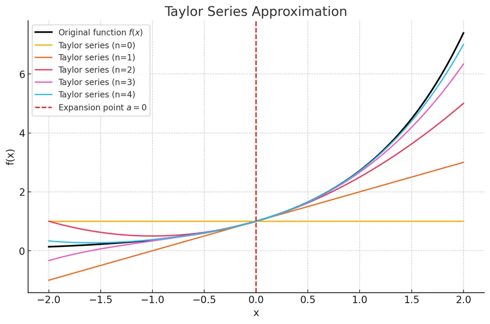
Near the point $x = a$, the partial sums of the Taylor series (called Taylor polynomials) provide increasingly accurate approximations to $f(x)$. This is often used in numerical methods to approximate complicated functions with simpler polynomial expressions.

II. Analysis of Behavior:

By examining the derivatives at a single point, one can gain insights into the function's local behavior, such as growth rates, curvature, and pattern of change.

III. Computational Efficiency:

In contexts like numerical analysis, physics, and engineering, it may be easier or more efficient to use a truncated Taylor series for computations instead of evaluating a complex function directly.

IV. Series Solutions to Differential Equations:

Many differential equations can be solved (or approximated) by expressing their solutions as Taylor series expansions.

Example

Taylor Series of $e^x$ at $a = 0$:

The exponential function $e^x$ has the unique property that all its derivatives are $e^x$ itself, and $e^0 = 1$. Thus:

$$ e^x = 1 + x + \frac{x^2}{2!} + \frac{x^3}{3!} + \cdots $$

This power series expansion converges for all real $x$, and even for complex $x$. Truncating the series after a few terms gives a good approximation of $e^x$ near $x = 0$.

Advantages

Representing functions as polynomials simplifies operations like integration, differentiation, and approximation, making complex functions easier to work with mathematically.
Taylor series provide a local approximation of functions by incorporating derivatives of all orders at a single point, capturing details such as slope, curvature, and higher-order behaviors.
The method offers a uniform approach to handling a wide range of functions, including transcendental functions like $\sin x$, $\cos x$, and $e^x$, through polynomial representations.

Limitations

The approximation has local validity, meaning it works best near the point $a$. Moving farther from $a$ can lead to reduced accuracy or even divergence.
Taylor series require infinite differentiability at the point $a$, limiting their applicability to functions that are not smooth or have points of non-differentiability.
Even for infinitely differentiable functions, convergence issues can arise, with some Taylor series converging only within a certain radius or failing to match the function outside that radius, affecting their global accuracy.