Constrained Optimization
Constrained optimization adds restrictions to the decision variables:
$$ \min_x f(x) $$
subject to
$$ g_i(x)\le0, \qquad h_j(x) = 0. $$
The constraints define the feasible set. A constrained optimum can lie on its boundary even when the objective gradient is nonzero.
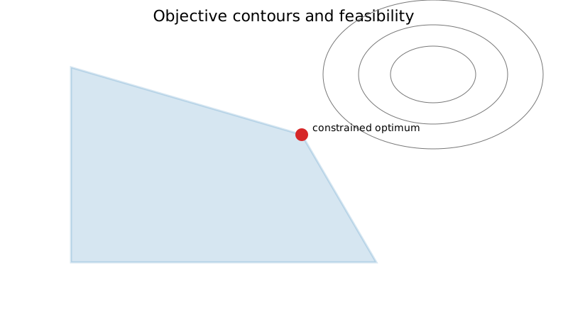
Equality constraints and tangency
For a single equality constraint
$$ h(x) = 0, $$
feasible first-order motions $d$ satisfy
$$ \nabla h(x)^\top d = 0. $$
At a regular constrained optimum, no feasible tangent direction can decrease the objective. Therefore the objective gradient must lie in the span of the constraint gradient:
$$ \nabla f(x^*) + \nu\nabla h(x^*) = 0. $$
This is the Lagrange-multiplier condition.
The equality multiplier $\nu$ can have either sign. Below, $\lambda_i$ is reserved for the nonnegative multipliers of inequalities written as $g_i\leq0$. Keeping those conventions separate makes the stationarity and sensitivity formulas consistent.
Inequality constraints
For an inequality $g_i(x)\le0$, the constraint is active at $x^*$ when $g_i(x^*)=0$. Inactive constraints have local slack and need not influence the stationarity condition.
This distinction is captured by complementary slackness:
$$ \lambda_i g_i(x^*) = 0. $$
KKT conditions
Define the Lagrangian
$$ \mathcal{L}(x,\lambda,\nu) = f(x) + \sum_i\lambda_i g_i(x) + \sum_j\nu_j h_j(x). $$
Under a suitable constraint qualification, a local optimum must satisfy
$$ \nabla_x\mathcal{L}(x^*,\lambda^*,\nu^*) = 0, $$
$$ g_i(x^*)\le0, \qquad h_j(x^*) = 0, $$
$$ \lambda_i^*\ge0, $$
and
$$ \lambda_i^*g_i(x^*) = 0. $$
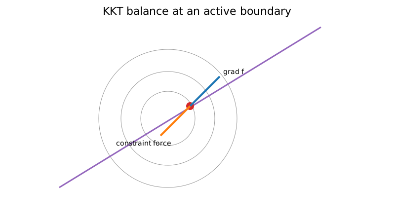
For a differentiable convex problem with convex inequalities and affine equalities, these conditions are sufficient for global optimality. A standard qualification is needed to ensure that an optimum has suitable multipliers, rather than to verify a supplied KKT certificate.
See Lagrange multipliers and KKT conditions for a detailed derivation.
Linear programming
When both the objective and constraints are linear, the problem becomes a linear program. The feasible set is a polyhedron, and in standard form with nonnegative variables, an attained finite optimum can be represented by an optimal extreme point. A general polyhedron with lineality need not have any extreme points.
The repository includes a compact two-phase simplex implementation that handles negative right-hand sides, equality constraints, and reports infeasible and unbounded problems. See linear programming.
Numerical KKT systems
Equality-constrained Newton and SQP-type methods lead to saddle-point linear systems of the form
$$ \begin{bmatrix} H & J_h^\top\\ J_h & 0 \end{bmatrix} \begin{bmatrix} p\\ \Delta\nu \end{bmatrix} {}= -\begin{bmatrix} \nabla f+J_h^\top\nu\\ h(x) \end{bmatrix}. $$
These systems can become ill-conditioned when constraint gradients are nearly dependent or when the problem is poorly scaled.
The repository's equality-constrained routine solves exactly this system with $H$ equal to the Hessian of the Lagrangian (analytic if provided, otherwise a central-difference estimate), starting from a least-squares multiplier estimate, and reduces the step length until the KKT residual decreases. Near a regular solution this gives quadratic convergence. Production solvers add Hessian modification for indefinite $H$, merit functions, and inequality handling, which this compact routine omits.
Deriving the equality KKT linear system
Collect the equality stationarity and feasibility equations into
$$ F(x,\nu)=\begin{bmatrix}\nabla f(x)+J_h(x)^\top\nu\\h(x)\end{bmatrix}. $$
Its Jacobian with respect to $(x,\nu)$ is exactly the displayed block matrix, with $H=\nabla_{xx}^2\mathcal L$ and rows of $J_h$ equal to the constraint gradients. Newton linearization $F+DF\,(p,\Delta\nu)=0$ gives the saddle-point solve. The lower block makes the step satisfy $h(x)+J_hp=0$, which enforces the linearized constraints; nonlinear constraints are generally not exactly satisfied after one step.
Quadratic local convergence requires a nonsingular KKT Jacobian, sufficiently smooth derivatives, accurate linear solves, and eventual acceptance of full steps. Nearly dependent constraint gradients can make this system sensitive even if the objective Hessian is well conditioned. A line search on the KKT residual helps control the iteration but does not by itself prove global convergence or classify the stationary point as a minimum.
Worked example
Minimize
$$ f(x,y) = x^2 + y^2 $$
subject to
$$ x + y = 4. $$
The Lagrangian is
$$ \mathcal{L} = x^2 + y^2 + \nu(x + y - 4). $$
Stationarity gives
$$ 2x + \nu = 0, \qquad 2y + \nu = 0, $$
so $x=y$. The constraint then gives
$$ x = y = 2. $$
The constrained minimum is therefore
$$ f(2,2) = 8. $$
Here $\nu=-4$. Parameterizing the constraint by $x=2+t$, $y=2-t$ gives $f=8+2t^2\geq8$, directly verifying global minimality along the feasible line. Equivalently, the objective Hessian $2I$ is positive definite on every nonzero tangent direction $(d,-d)$.
Feasibility and scaling
In practice, monitor both optimality and feasibility. A point with a tiny gradient can still be unacceptable if constraints are violated.
Useful residuals include
$$ r_{\text{eq}} = \| h(x)\|, $$
$$ r_{\text{ineq}} = \|\max(g(x),0)\|, $$
and the stationarity residual
$$ r_{\text{stat}} = \|\nabla_x\mathcal{L}\|. $$