Convex Optimization

Convex optimization minimizes a convex objective over a convex feasible set. Its structure provides a useful guarantee before an algorithm is chosen: a point that is locally optimal is also globally optimal. Supporting-hyperplane inequalities and, when applicable, KKT multipliers turn that geometric property into conditions that can be checked mathematically. The central statement is:

For a convex objective over a convex feasible set, every local minimum is global.

That fact turns first-order or KKT conditions into global certificates of optimality.

Convex sets

A set $C\subseteq\mathbb{R}^n$ is convex if

$$ \theta x + (1 - \theta)y\in C $$

for every $x,y\in C$ and every $\theta\in[0,1]$.

Examples include affine subspaces, half-spaces, Euclidean balls, boxes, and polyhedra.

Convex functions

A function $f$ is convex when

$$ f(\theta x + (1 - \theta)y) \le \theta f(x) + (1 - \theta)f(y). $$

Geometrically, the chord between two points on the graph lies above the graph.

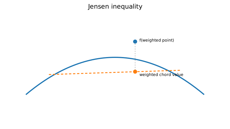
For differentiable $f$, convexity is equivalent to the global first-order lower bound

$$ f(y)\ge f(x) + \nabla f(x)^\top(y - x). $$

For twice-differentiable $f$ on a convex domain, a sufficient and necessary condition is

$$ \nabla^2 f(x)\succeq0 $$

for every $x$ in the domain.

Why every local minimum is global

Suppose $x^*$ were a local minimum but a feasible $y$ had $f(y)<f(x^*)$. Convexity of the feasible set keeps $x_\theta=(1-\theta)x^*+\theta y$ feasible, and convexity of the objective gives

$$ f(x_\theta)\leq(1-\theta)f(x^*)+\theta f(y)<f(x^*) $$

for every $0<\theta\leq1$. Taking $\theta$ arbitrarily small contradicts local minimality. This proof depends on both convexity assumptions.

For a differentiable convex objective on a convex feasible set $C$, optimality is equivalent to

$$ \nabla f(x^*)^\top(y-x^*)\geq0\qquad\text{for every }y\in C. $$

Sufficiency follows directly from the first-order lower bound. In an unconstrained domain this reduces to $\nabla f(x^*)=0$; at a boundary it generally does not.

Strong convexity

A differentiable function is $\mu$-strongly convex if

$$ f(y)\ge f(x) + \nabla f(x)^\top(y - x) + \frac{\mu}{2}\| y - x\|_2^2. $$

For $\mu>0$, strong convexity implies that a minimizer, if it exists, is unique and enables explicit convergence-rate bounds for first-order methods. A continuous strongly convex function on all of $\mathbb R^n$ attains its minimum; on a restricted nonclosed domain, attainment must be checked separately.

Smoothness and conditioning

If the gradient is $L$-Lipschitz,

$$ \|\nabla f(x) - \nabla f(y)\|_2\le L\| x - y\|_2, $$

then gradient descent with step $1/L$ satisfies standard convergence guarantees. When $f$ is both $\mu$-strongly convex and $L$-smooth, the ratio

$$ \kappa = \frac{L}{\mu} $$

plays the role of a condition number.

Convex constrained problems

A standard convex problem has the form

$$ \min_x f(x) $$

subject to

$$ g_i(x)\le0, \qquad Ax = b, $$

where $f$ and every $g_i$ are convex and the equality constraints are affine.

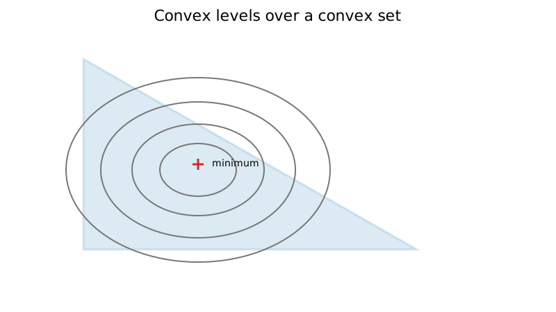
Under a suitable constraint qualification such as Slater's condition, the KKT conditions are necessary and sufficient for optimality.

For a differentiable convex problem, any point and multipliers satisfying KKT already certify global optimality. A qualification such as Slater’s condition is used to guarantee the existence of such multipliers at an optimum. One common form of Slater’s condition asks for a point in the relative interior of the domain that satisfies the affine equalities and all inequalities strictly.

Quadratic programming

A convex quadratic program has objective

$$ q(x) = \frac12 x^\top Qx + c^\top x $$

with

$$ Q\succeq0. $$

The repository implementation checks the eigenvalues of $Q$ and then uses a projected-gradient style iteration. See quadratic programming for details.

Convexity checks in computation

Randomly testing Jensen's inequality at sampled points can find violations, but passing random tests does not prove convexity. Analytical structure is preferable:

• known convex atoms and composition rules;
• Hessian positive semidefiniteness;
• epigraph arguments;
• transformations that preserve convexity.

The repository's is_convex_function helper should therefore be read as a numerical diagnostic, not a proof.

Worked example

Consider

$$ f(x,y) = x^2 + 4y^2 + 2x - 8y. $$

Its Hessian is

$$ H= \begin{bmatrix} 2&0\\ 0&8 \end{bmatrix}\succ0, $$

so the function is strongly convex. Setting the gradient to zero gives

$$ 2x + 2 = 0, \qquad 8y - 8 = 0, $$

hence

$$ (x^*,y^*) = (-1,1). $$

Because the objective is convex, this stationary point is automatically the unique global minimum.

Modeling lessons

Before choosing a generic nonlinear solver, ask whether the problem can be expressed as a convex one. A correct convex formulation can transform an apparently difficult search problem into one with global guarantees and reliable numerical methods.