Lagrange Multipliers and KKT Conditions

Lagrange multipliers convert constrained first-order optimality into a system of equations involving the objective and constraint gradients.

Equality constraint

Consider

$$ \min_x f(x) $$

subject to

$$ h(x) = 0. $$

At a regular constrained optimum, the objective gradient is normal to the feasible tangent space, so

$$ \nabla f(x^{\ast}) + \nu\nabla h(x^*) = 0. $$

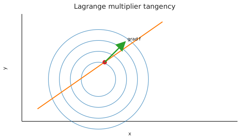
The Lagrangian is

$$ \mathcal{L}(x,\nu) = f(x) + \nu h(x). $$

The first-order equations are

$$ \nabla_x\mathcal{L} = 0, \qquad h(x) = 0. $$

Multiple constraints

With equality constraints $h_j(x)=0$ and inequalities $g_i(x)\le0$,

$$ \mathcal{L}(x,\lambda,\nu) = f(x) + \sum_i\lambda_i g_i(x) + \sum_j\nu_j h_j(x). $$

The Karush-Kuhn-Tucker conditions are:

Stationarity

$$ \nabla_x\mathcal{L} = 0. $$

Primal feasibility

$$ g_i(x)\le0, \qquad h_j(x) = 0. $$

Dual feasibility

$$ \lambda_i\ge0. $$

Complementary slackness

$$ \lambda_i g_i(x) = 0. $$

Active constraints

Complementary slackness says that either

$$ g_i(x^*)<0\quad\Rightarrow\quad\lambda_i = 0, $$

or the constraint is active:

$$ g_i(x^*) = 0. $$

Only active inequality constraints can exert a first-order force on the optimum.

Constraint qualifications

KKT conditions are not automatically necessary at every constrained optimum. Regularity assumptions are needed to rule out degenerate constraint geometry. Common examples include LICQ and Slater's condition in convex optimization.

Regularity and second-order conditions

LICQ means that the gradients of all equalities and active inequalities are linearly independent at the candidate point. It makes the normal-direction description well behaved. Without a qualification, a true optimum need not have KKT multipliers: minimize $f(x)=x$ subject to $h(x)=x^2=0$. The only feasible point is zero, but stationarity would require $1+\nu\cdot0=0$, which is impossible.

For an equality-constrained problem at a regular stationary point, the Hessian of the Lagrangian, not just the objective, controls curvature along feasible tangent directions. The necessary condition is $d^\top\nabla_{xx}^2\mathcal L\,d\geq0$ for every $d$ satisfying $J_hd=0$. Strict positivity for every nonzero such direction is a sufficient local-minimum condition under the usual smoothness assumptions. With inequalities, the corresponding second-order test uses the appropriate critical cone.

Worked inequality and multiplier sign

Minimize $(x-2)^2$ subject to $g(x)=x-1\leq0$. The unconstrained minimizer is infeasible, so the constrained solution is $x^*=1$. Stationarity gives $2(1-2)+\lambda=0$, hence $\lambda=2\geq0$, and complementary slackness holds because $g(1)=0$.

If the upper bound becomes $b$ near $1$, the optimal value is $V(b)=(b-2)^2$, so $V'(1)=-2=-\lambda$. Increasing the upper bound relaxes the constraint and lowers the value. An active constraint may also have multiplier zero: minimize $x^2$ subject to $-x\leq0$ at $x=0$. Activity permits a nonzero multiplier but does not require one.

For a differentiable convex objective, convex inequalities, and affine equalities, KKT is sufficient without an additional qualification: stationarity minimizes the convex Lagrangian, dual feasibility makes it a lower bound on feasible objectives, and complementary slackness makes the bound exact. Qualifications establish necessity and multiplier existence. See Boyd and Vandenberghe, Convex Optimization, Chapter 5, for the duality framework.

Sensitivity interpretation

Lagrange multipliers often measure how the optimal value changes when a constraint right-hand side is perturbed. This is the origin of the “shadow price” interpretation in economics and operations research.

The sign depends on how the constraint is parameterized, so sensitivity formulas should be derived from the chosen Lagrangian rather than memorized without context.

KKT residuals

Numerically, it is useful to monitor a combined residual such as

$$ r= \begin{bmatrix} \nabla_x\mathcal{L}\\ h(x) \end{bmatrix} $$

for equality-constrained problems. The repository implementation applies Newton's method to this residual: each step solves the KKT system with the Hessian of the Lagrangian $\nabla^2f+\sum_j\nu_j\nabla^2h_j$ (supplied analytically or estimated by finite differences), and a backtracking search on the residual norm globalizes the iteration. When this iteration converges to a zero residual, it reaches a KKT point, which need not be a minimizer; the second-order conditions must be checked separately.