Simulated Annealing
Simulated annealing is a stochastic global-search method that occasionally accepts worse moves so that it can escape local minima.
Acceptance rule
Suppose the current point is $x$ and a candidate $y$ has objective difference
$$ \Delta f = f(y) - f(x). $$
If $\Delta f\le0$, accept the candidate. If $\Delta f>0$, accept with probability
$$ P = \exp\left(-\frac{\Delta f}{T}\right), $$
where $T>0$ is the temperature.
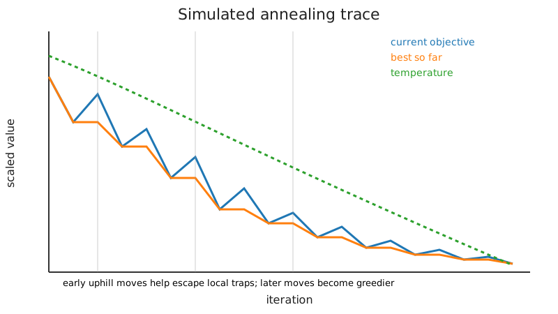
At high temperature, uphill moves are common. At low temperature, the method becomes increasingly greedy.
Why the exponential acceptance rule appears
At a fixed temperature, the Boltzmann target has weights $\pi_T(x)\propto e^{-f(x)/T}$. With a symmetric proposal $q(y\mid x)=q(x\mid y)$, the Metropolis probability is
$$ \min\left(1,\frac{\pi_T(y)}{\pi_T(x)}\right)=\min(1,e^{-\Delta f/T}), $$
which satisfies detailed balance. For an asymmetric proposal, the corresponding Metropolis–Hastings ratio also contains $q(x\mid y)/q(y\mid x)$. Cooling changes the target over time, so fixed-temperature sampling arguments alone do not prove annealing convergence.
The normalization constant of the Boltzmann distribution cancels in the acceptance ratio, so it need not be computed. Adding a constant to every objective value also leaves $\Delta f$ unchanged; multiplying the objective by a positive constant instead changes the temperature scale needed for the same acceptance probabilities.
For a representative uphill cost $\Delta f=1$, the acceptance probabilities are about $0.905$ at $T=10$, $0.368$ at $T=1$, and $4.54\times10^{-5}$ at $T=0.1$. Temperature has the same scale as the objective: multiplying $f$ by $a>0$ requires multiplying $T$ by $a$ to retain the same acceptance probabilities.
For numerical stability, an uphill proposal can be accepted when $\log U<-\Delta f/T$ for $U$ uniform on $(0,1)$. This avoids explicitly forming a very small exponential.
Cooling schedule
The repository uses geometric cooling:
$$ T_{k+1} = \alpha T_k, \qquad 0<\alpha<1. $$
The temperature is lowered after every proposal, so after $k$ iterations $T_k=\alpha^kT_0$. The choice of $T_0$, $\alpha$, proposal scale, and iteration budget all matter.
Other common schedules include linear cooling, $T_k=T_0(1-k/K)$, and logarithmic cooling, $T_k=c/\ln(k+2)$, for which classical finite-state convergence results hold under appropriate connectivity assumptions when $c$ is at least the critical energy-barrier depth. Continuous spaces and different proposal mechanisms require their own assumptions; the formula alone is not a universal guarantee.
Proposal distribution
For continuous variables, a simple proposal is
$$ y = x + \sigma z, \qquad z\sim\mathcal N(0,I). $$
Candidates are clipped to the box bounds in the repository implementation.
Clipping changes proposal probabilities near the boundary, so the proposal is generally no longer symmetric there. The simple acceptance rule remains a search heuristic in this implementation; the symmetric-proposal Boltzmann argument should not be transferred to clipped moves without analyzing the resulting proposal law.
If $\sigma$ is too small, the chain explores slowly. If it is too large, most proposals land in poor regions and are rejected after the temperature cools.
Best-so-far versus current state
The current state can move uphill, so the algorithm separately tracks the best point seen. This distinction is essential: the final state is not necessarily the best state visited.
Convergence theory versus practical schedules
Classical convergence proofs require logarithmic cooling, which is far slower than the schedules used in most practical code. Geometric cooling is popular because it reaches a useful low-temperature regime quickly, but it trades theoretical guarantees for finite-time performance.
For the assumptions behind the logarithmic barrier-depth result, see Hajek, Cooling Schedules for Optimal Annealing (1988). These are asymptotic convergence statements and do not supply a finite run length at which a particular continuous search must find the optimum.
Reproducibility
Because the path is random, report the seed and preferably repeat the run over multiple seeds. For comparisons, summarize distributions of final objective values rather than showing only the best lucky run.