Optimization
Optimization asks a simple question with many numerical subtleties:
Among all admissible choices, which one gives the smallest (or largest) objective value?
A minimization problem is written as
$$ \min_{x\in\Omega} f(x), $$
where $x\in\mathbb{R}^n$ is the decision vector, $f$ is the objective, and $\Omega$ is the feasible set. Maximization can always be rewritten as minimization of $-f$.
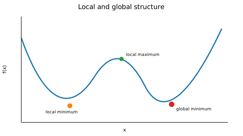
The difficulty of an optimization problem depends less on its dimension alone than on its geometry: convexity, smoothness, conditioning, constraints, and the number of local minima all determine which algorithms are appropriate.
A useful classification
| Property | Typical consequence | Common methods |
|---|---|---|
| smooth, unconstrained, convex | every local minimum is global | gradient, Newton, BFGS |
| smooth, unconstrained, non-convex | stationary points may be minima, maxima, or saddles | local methods with safeguards, multi-start |
| constrained | iterates must respect or penalize feasibility | projected methods, active-set, KKT, SQP |
| derivative-free / black-box | gradients may be unavailable or unreliable | grid search, simulated annealing, evolutionary methods |
| multimodal | many local minima compete | global or stochastic search |
The existing implementation chapter is organized around four broad families:
Detailed notes cover the algorithms inside those families:
- Line search
- Newton and quasi-Newton methods
- Linear programming
- Lagrange multipliers and KKT conditions
- Quadratic programming
- Simulated annealing
- Genetic algorithms
For basic steepest descent, see the earlier gradient descent note.
First-order optimality
For an unconstrained differentiable objective, a local minimizer $x^*$ in the interior must satisfy
$$ \nabla f(x^*) = 0. $$
This condition is necessary, not sufficient. A stationary point can also be a maximum or saddle point.
For a twice-differentiable function, the Hessian
$$ H(x) = \nabla^2 f(x) $$
helps classify a stationary point. If $H(x^*)$ is positive definite, $x^*$ is a strict local minimum. If it is negative definite, $x^*$ is a strict local maximum. An indefinite Hessian indicates a saddle.
What a singular Hessian does and does not tell us
At an interior local minimum, a twice-differentiable objective has zero gradient and positive-semidefinite Hessian. Positive definiteness is a sufficient condition for a strict local minimum, but it is not necessary. In one dimension, $x^4$, $-x^4$, and $x^3$ all have zero first and second derivatives at zero, yet zero is respectively a minimum, a maximum, and neither. A semidefinite or zero Hessian therefore requires higher-order or direct analysis.
Existence is a separate question. A continuous objective on a nonempty compact feasible set attains a minimum. Without such a condition, the infimum may not be attained, as with $f(x)=e^x$ on $\mathbb R$, or the objective may be unbounded below. An algorithm cannot return an attained optimum when the mathematical problem has none.
Why conditioning matters
Consider the quadratic
$$ f(x) = \frac12 x^\top A x - b^\top x, $$
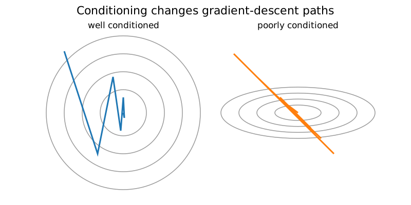
with $A$ symmetric positive definite. Its contours are ellipses, and the condition number
$$ \kappa_2(A) = \frac{\lambda_{\max}(A)}{\lambda_{\min}(A)} $$
measures their elongation.
When $\kappa_2(A)$ is large, steepest descent tends to zig-zag across a narrow valley instead of moving directly toward the minimum.
For a quadratic, fixed-step gradient descent
$$ x_{k+1} = x_k - \alpha(Ax_k - b) $$
converges when
$$ 0<\alpha< \frac{2}{\lambda_{\max}(A)}. $$
With the best fixed step for the spectrum, the contraction factor depends on $\kappa$; poor conditioning directly slows convergence.
To derive the factor, subtract $Ax^*=b$ from the gradient update: $e_{k+1}=(I-\alpha A)e_k$. In an orthonormal eigenbasis each error component is multiplied by $1-\alpha\lambda_i$. Balancing the extreme factors gives
$$ \alpha_* = \frac{2}{\lambda_{\min}+\lambda_{\max}},\qquad q_* = \frac{\lambda_{\max}-\lambda_{\min}}{\lambda_{\max}+\lambda_{\min}}=\frac{\kappa-1}{\kappa+1}. $$
For large $\kappa$, this factor is close to one, so many small error reductions are needed. Variable scaling and preconditioning aim to improve that spectrum.
Local versus global guarantees
A local minimum $x^*$ satisfies
$$ f(x^*)\le f(x) $$
for all $x$ in some neighborhood of $x^*$. A global minimum satisfies the inequality for every feasible point.
Convexity bridges the two notions: if $f$ is convex and $\Omega$ is convex, every local minimum is global. Without convexity, a local solver can only guarantee convergence to a nearby stationary point under suitable assumptions.
Constraints change optimality conditions
For
$$ \min_x f(x) $$
subject to
$$ g_i(x)\le0, \qquad h_j(x) = 0, $$
we cannot generally set $\nabla f=0$. The gradient may point outside the feasible region. Instead, active constraint gradients enter through the Lagrangian and KKT conditions.
Choosing a method
A practical decision sequence is:
- Exploit structure first. Determine whether the problem is convex, quadratic, linear, separable, sparse, or otherwise special.
- Use derivatives when trustworthy. They usually reduce function evaluations dramatically.
- Scale variables and constraints. Poor scaling can mimic difficult geometry.
- Use globalization safeguards. Line search and trust-region ideas keep Newton-like methods from taking destructive steps far from a solution.
- Reserve global methods for genuinely multimodal problems. They are usually much more expensive.
- Verify the result. Inspect gradients, KKT residuals, feasibility, and sensitivity rather than relying only on a solver's success flag.
Stopping criteria
Common termination tests include
$$ \|\nabla f(x_k)\|\le\varepsilon_g, $$
$$ \| x_{k+1} - x_k\|\le\varepsilon_x(1 + \| x_k\|), $$
and
$$ |f(x_{k+1}) - f(x_k)|\le\varepsilon_f(1 + |f(x_k)|). $$
No single criterion is reliable in every problem. Small steps can occur because of a bad step size, and a small objective change can occur on a flat plateau even when the gradient is not small.