Local Optimization

Local optimization methods refine a starting point using information about the objective near the current iterate. They are the default tools for smooth numerical optimization because they can converge rapidly with far fewer evaluations than global search.

The tradeoff is fundamental: on a non-convex objective, the answer may depend on the initial point.

Descent directions

For a differentiable objective, a vector $p_k$ is a descent direction at $x_k$ if

$$ \nabla f(x_k)^\top p_k<0. $$

An update has the generic form

$$ x_{k+1} = x_k + \alpha_k p_k, $$

where $\alpha_k>0$ is the step length.

Steepest descent chooses

$$ p_k = -\nabla f(x_k). $$

Newton's method solves

$$ \nabla^2 f(x_k)p_k = -\nabla f(x_k), $$

and BFGS uses an approximate inverse Hessian $H_k$:

$$ p_k = -H_k\nabla f(x_k). $$

Checking that a direction really descends

Taylor expansion along $p$ gives $f(x+\alpha p)=f(x)+\alpha\nabla f(x)^\top p+o(\alpha)$ as $\alpha\to0^+$. A negative directional derivative therefore guarantees improvement for a sufficiently small positive step, although it does not establish that a full step is safe.

For steepest descent, $g^\top p=-\|g\|_2^2<0$ whenever $g\ne0$. For Newton with a positive-definite Hessian $B$, $p=-B^{-1}g$ gives $g^\top p=-g^\top B^{-1}g<0$. The same argument applies to BFGS when its inverse approximation is positive definite. An indefinite curvature matrix removes this guarantee and explains the need for safeguards.

At convergence, a small gradient establishes approximate stationarity, rather than a global or even local minimum by itself. In constrained problems the appropriate test is a projected-gradient or KKT residual, since the ordinary gradient need not vanish at a boundary optimum.

The Rosenbrock valley

The Rosenbrock function

$$ f(x,y) = (1 - x)^2 + 100(y - x^2)^2 $$

has a unique global minimum at $(1,1)$, but its narrow curved valley makes it difficult for methods that do not account for curvature.

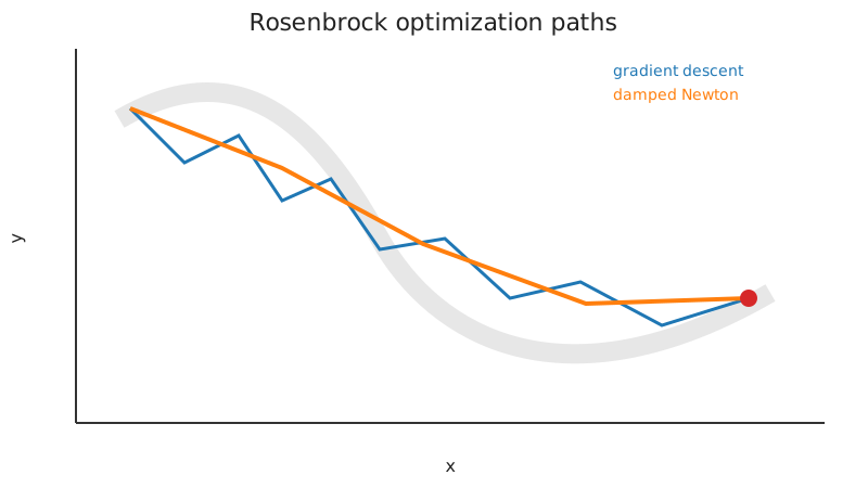
Gradient descent makes inexpensive iterations but often zig-zags. Newton and quasi-Newton methods spend more work per iteration to learn the valley geometry.

Convergence rates

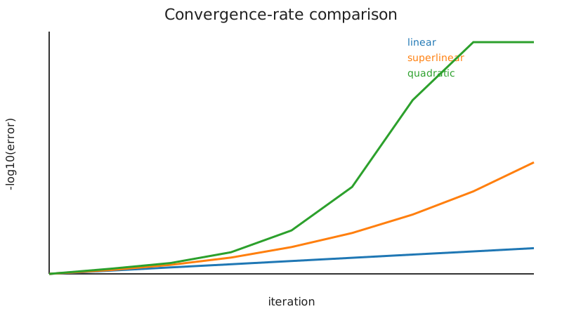
Near a sufficiently regular minimizer, common asymptotic rates are:

• gradient descent: linear under strong convexity with a suitable step size;
• BFGS: often superlinear with a suitable line search;
• Newton: quadratic when the Hessian is nonsingular and the iterate is sufficiently close.

If $e_k=\|x_k-x^*\|$, these idealized rates look like

$$ e_{k+1}\le c e_k, $$

$$ \frac{e_{k+1}}{e_k}\to0, $$

and

$$ e_{k+1}\le c e_k^2, $$

respectively.

For linear convergence the factor satisfies $0<c<1$. In the quadratic bound, a fixed positive constant need not be below one: it is the square of an already small error that gives the rapid reduction. These are local, asymptotic statements. Since the true minimizer is usually unknown during a solve, practical diagnostics use gradients, accepted steps, and residuals rather than assuming that the error $e_k$ is directly observable.

Why plain Newton can fail

The Newton direction is not guaranteed to be a descent direction when the Hessian is indefinite. Far from a minimizer it can point toward a maximum, a saddle, or simply take an enormous step.

Practical Newton-type solvers therefore use one or more safeguards:

• line search;
• Hessian modification or damping;
• trust regions;
• quasi-Newton positive-definite approximations.

The repository implementation intentionally keeps the algorithms compact: fixed-step gradient descent, plain Newton using numpy.linalg.solve, and BFGS with a strong Wolfe line search (bracketing followed by bisection zoom, see line search).

BFGS update

Define

$$ s_k = x_{k+1} - x_k, \qquad y_k = \nabla f(x_{k+1}) - \nabla f(x_k), $$

and

$$ \rho_k = \frac{1}{y_k^\top s_k}. $$

The inverse-Hessian BFGS update is

$$ H_{k+1} = (I - \rho_k s_k y_k^\top)H_k(I - \rho_k y_k s_k^\top) + \rho_k s_k s_k^\top. $$

If $H_k$ is positive definite and $y_k^\top s_k>0$, the update preserves positive definiteness.

See Newton and quasi-Newton methods for the derivation and numerical interpretation.

Worked quadratic example

For

$$ f(x,y) = \frac12(8x^2 + 2y^2) - 4x - 2y, $$

we have

$$ \nabla f= \begin{bmatrix} 8x-4\\ 2y-2 \end{bmatrix}, \qquad H= \begin{bmatrix} 8&0\\ 0&2 \end{bmatrix}. $$

The minimizer solves $H x=b$:

$$ (x^{\ast}, y^{\ast}) = (0.5, 1). $$

Newton reaches it in one exact step from any starting point because the quadratic model is the function itself. Gradient descent generally needs multiple steps and its rate is controlled by the eigenvalue ratio $8/2=4$.

Practical diagnostics

For a local solver, report more than the final point. Useful diagnostics include:

• gradient norm;
• objective reduction;
• accepted step lengths;
• number of function and gradient evaluations;
• Hessian eigenvalues or quasi-Newton curvature tests;
• sensitivity to the starting point.