Newton and Quasi-Newton Methods
Newton-type methods use local curvature to transform the gradient into a better-scaled search direction.
Newton step
At $x_k$, approximate the objective by its quadratic Taylor model
$$ m_k(p) = f(x_k) + g_k^\top p + \frac12 p^\top B_kp, $$
where
$$ g_k = \nabla f(x_k), \qquad B_k = \nabla^2 f(x_k). $$
Setting the gradient of the model to zero gives
$$ B_kp_k = -g_k. $$
The implementation should solve this linear system; it should not explicitly form $B_k^{-1}$.
Why Newton can converge quadratically
Near a nondegenerate minimizer, the Hessian changes smoothly and the quadratic model becomes highly accurate. Under standard assumptions,
$$ \|x_{k+1}-x^*\|_2\leq C\|x_k-x^*\|_2^2 $$
This rapid local convergence is the main attraction of Newton's method.
A more explicit quadratic-convergence argument
Let $x^*$ have zero gradient and nonsingular Hessian, write $e=x-x^*$, and let $B(x)=\nabla^2 f(x)$. The fundamental theorem of calculus along the segment gives
$$ \nabla f(x)=\int_0^1B(x^*+te)e\,dt. $$
A full Newton step therefore has error
$$ e_{\mathrm{new}}=B(x)^{-1}\int_0^1[B(x)-B(x^*+te)]e\,dt. $$
If $B$ is locally Lipschitz with constant $M$ and $\|B(x)^{-1}\|\leq K$ nearby, then $\|e_{\mathrm{new}}\|\leq KM\|e\|^2/2$. Starting sufficiently close keeps the iteration in this neighborhood. This proves a local quadratic bound; damped steps, inaccurate derivatives, or an indefinite stationary point require separate interpretation.
In the quadratic model, setting the model gradient to zero identifies its minimizer only when its Hessian is positive definite. Throughout this note, $B_k$ denotes a Hessian or Hessian approximation, while $H_k$ denotes an inverse-Hessian approximation. Keeping these roles distinct avoids applying an inverse update to a Hessian matrix by mistake.
Indefinite Hessians
If $B_k$ is indefinite, the Newton direction can satisfy
$$ g_k^\top p_k>0, $$
meaning it is an ascent direction. Modified Newton methods alter the Hessian or use a trust region to recover a reliable step.
Quasi-Newton idea
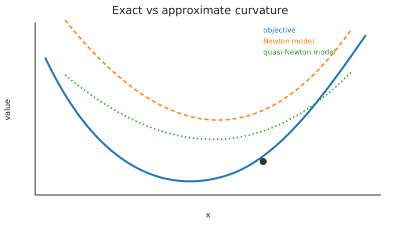
Quasi-Newton methods avoid exact second derivatives. Instead they build a matrix approximation from changes in iterates and gradients:
$$ s_k = x_{k+1} - x_k, \qquad y_k = g_{k+1} - g_k. $$
The secant equation is
$$ B_{k+1}s_k = y_k. $$
It is the multidimensional analogue of replacing a derivative by a finite secant slope.
BFGS
For an inverse-Hessian approximation $H_k$, BFGS uses
$$ H_{k+1} = (I - \rho s y^\top)H_k(I - \rho y s^\top) + \rho ss^\top, $$
where
$$ \rho = \frac{1}{y^\top s}. $$
When $y^\top s>0$, positive definiteness is preserved. A line search satisfying the Wolfe curvature condition guarantees $y^\top s>0$ at every step, which is why BFGS is paired with a Wolfe line search rather than plain backtracking.
Verifying the BFGS secant equation
The gradient change is an averaged curvature action,
$$ y_k=\int_0^1\nabla^2f(x_k+ts_k)s_k\,dt, $$
which motivates $B_{k+1}s_k=y_k$, or equivalently $H_{k+1}y_k=s_k$. To check the inverse update, note that $(I-\rho ys^\top)y=0$ and $\rho ss^\top y=s$ because $\rho(y^\top s)=1$. Substitution gives $H_{k+1}y=s$ exactly.
For any vector $z$, the update also gives
$$ z^\top H_{k+1}z=w^\top H_kw+\rho(s^\top z)^2,\qquad w=(I-\rho ys^\top)z. $$
If $H_k\succ0$ and $y^\top s>0$, both terms are nonnegative and can vanish together only for $z=0$. Thus positive definiteness is preserved. When $y^\top s$ is tiny, computing its reciprocal can amplify rounding; skipping or damping the update is a numerical safeguard even when the exact curvature condition is positive.
Cost comparison
For a dense problem with $n$ variables:
- exact Hessian storage costs $O(n^2)$;
- a dense Newton solve costs about $O(n^3)$;
- dense BFGS stores $O(n^2)$ but avoids explicit second derivatives;
- limited-memory BFGS reduces storage to $O(mn)$ using only recent update pairs.
When to prefer each method
Use Newton when accurate Hessians are affordable and the problem is not too large. Use BFGS when gradients are available but Hessians are inconvenient. For very large problems, prefer sparse Newton-Krylov or limited-memory variants.