Linear Programming

A linear program optimizes a linear objective over linear constraints. A common minimization form is

$$ \min_x c^\top x $$

subject to

$$ Ax\le b, \qquad x\ge0. $$

The feasible region is a polyhedron.

Why vertices matter

For a feasible linear program in the nonnegative-variable form above, an attained finite optimum has an optimal extreme point. The unrestricted statement needs care: a polyhedron containing lines may have no vertices, even when a finite optimal value is attained. In two dimensions these are polygon vertices.

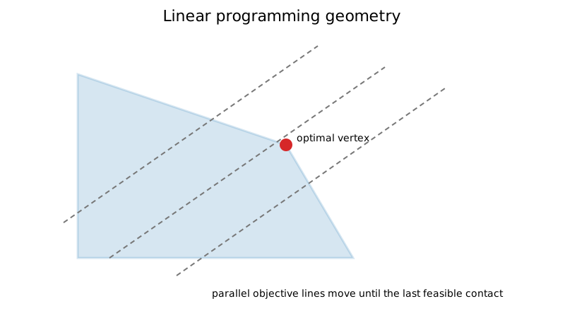
The objective contours

$$ c^\top x = \gamma $$

are parallel hyperplanes. Moving them in the improving direction until they last touch the feasible region reveals the optimum geometrically.

Slack variables

An inequality

$$ a_i^\top x\le b_i $$

can be rewritten as

$$ a_i^\top x + s_i = b_i, \qquad s_i\ge0. $$

Slack variables convert the inequalities into equalities while measuring unused capacity.

Simplex idea

The simplex method maintains a basis corresponding to a basic feasible solution and moves between adjacent vertices.

For minimization, reduced costs indicate whether introducing a nonbasic variable can improve the objective. If all reduced costs satisfy the optimality sign convention, the current basis is optimal.

A ratio test chooses the leaving variable so that feasibility is preserved.

Reduced costs and the ratio test

In equality standard form $A_Bx_B+A_Nx_N=b$, choose an invertible basis matrix $B=A_B$ and set the nonbasic variables to zero. The basic point is feasible when $x_B=B^{-1}b\geq0$. Increasing nonbasic variable $x_j$ by $\theta\geq0$ changes the basic variables to

$$ x_B(\theta)=B^{-1}b-\theta B^{-1}A_j. $$

The objective changes by $\theta\overline c_j$, where

$$ \overline c_j=c_j-c_B^\top B^{-1}A_j $$

is the reduced cost. For minimization, a negative reduced cost is an improving candidate. Let $d=B^{-1}A_j$. Feasibility requires $\theta\leq(x_B)_i/d_i$ wherever $d_i>0$; the minimum of these ratios identifies a leaving variable. If no component of $d$ is positive, that feasible direction permits unbounded improvement. A zero minimum ratio is a degenerate pivot and may change the basis without changing the point or objective.

These formulas use inverse notation to derive the relationships; implementations can obtain the quantities by factorization solves. Phase I is needed when an initial feasible basis is unavailable, because the ratio test preserves existing feasibility rather than creating it from an arbitrary point.

Unboundedness and infeasibility

A correct LP solver must distinguish:

• optimal: a feasible point achieves the best finite value;
• unbounded: feasible points can improve the objective without limit;
• infeasible: no point satisfies all constraints.

The repository's linear_programming implements the two-phase simplex method for

$$ \min c^\top x\quad\text{s.t.}\quad A_{\text{ub}}x\le b_{\text{ub}},\; A_{\text{eq}}x=b_{\text{eq}},\; x\ge0. $$

A constraint $a^\top x\ge\beta$ is passed as $-a^\top x\le-\beta$.

• Phase I. Rows whose slack variable cannot start in the basis (negative right-hand side after adding slacks, or equalities) get an artificial variable $t_i\ge0$. Phase I minimizes $\sum_it_i$. If the optimum is positive, no feasible point exists and a ValueError ("infeasible") is raised. Otherwise the final basis is a basic feasible solution; artificial variables left in the basis at level zero are pivoted out, and rows that are linear combinations of others are dropped.
• Phase II. The original objective is priced out against that basis and ordinary simplex pivots run. If an entering column has no positive entry, the problem is unbounded and a ValueError ("unbounded") is raised.

Pivoting uses Dantzig's most-negative-reduced-cost rule and switches to Bland's smallest-index rule after a run of degenerate pivots to avoid cycling. Results agree with scipy.optimize.linprog on randomized test problems with mixed-sign right-hand sides. It remains a dense-tableau teaching solver, not a production code.

Worked example

Maximize

$$ 5x_1 + 4x_2 $$

subject to

$$ 2x_1 + x_2\le8, $$

$$ x_1 + 2x_2\le7, $$

$$ x_1,x_2\ge0. $$

The boundary intersection solves

$$ 2x_1 + x_2 = 8, $$

$$ x_1 + 2x_2 = 7, $$

which gives

$$ (x_1,x_2) = (3,2). $$

The objective value is

$$ 5(3) + 4(2) = 23, $$

larger than at the other feasible vertices.

The other vertices are $(0,0)$, $(4,0)$, and $(0,3.5)$, with values $0$, $20$, and $14$. A dual certificate also proves optimality without enumerating vertices: multiply the first inequality by $2$ and the second by $1$. Adding gives $5x_1+4x_2\leq2(8)+7=23$, attained at $(3,2)$. To pass this maximization to a minimization interface, use objective vector $c=(-5,-4)$.

Numerical notes

Degeneracy can produce zero-length pivots and cycling. Real solvers use anti-cycling rules, presolve, scaling, sparse linear algebra, and often dual-simplex or interior-point variants.