Chi-Square Tests and Categorical Data Analysis
The chi-square ($\chi^2$) test is a family of statistical tests for categorical count data. These tests compare observed frequencies with the frequencies expected under a null hypothesis.
A large difference between observed and expected counts provides evidence that the null hypothesis may not adequately explain the data.
Types of Chi-Square Tests:
- The goodness-of-fit test determines whether the distribution of one categorical variable follows a specified distribution.
- The test of homogeneity assesses whether several populations or groups have the same distribution of a categorical variable.
- The test of independence evaluates whether two categorical variables are associated within a population.
Although these tests address different questions, they use the same basic idea:
Categorical Data
Categorical data consist of observations classified into groups or categories rather than measured on a numerical scale.
Categorical variables may be:
- nominal, where categories have no natural ordering, or
- ordinal, where categories have a meaningful ordering.
For a single categorical variable, each observation belongs to one category. When several categorical variables are recorded, each observation belongs to one category for each variable.
For example, consider Titanic passengers classified by survival status and ticket class:
- Survival status: Survived or Died.
- Ticket class: First Class, Second Class, Third Class, or Crew.
Each passenger has one survival status and one ticket-class category.
Contingency Tables
A contingency table, also called a cross-tabulation or crosstab, summarizes counts for combinations of categorical variables.
For example, Titanic survival data can be represented in a $2\times4$ contingency table:
| First Class | Second Class | Third Class | Crew | Total | |
|---|---|---|---|---|---|
| Survived | $a$ | $b$ | $c$ | $d$ | $S$ |
| Died | $e$ | $f$ | $g$ | $h$ | $D$ |
| Total | 325 | 285 | 706 | 885 | 2,201 |
Here, $a$ through $h$ represent the observed counts in each cell.
The row and column totals are called marginal totals. They are used to calculate expected counts in tests of homogeneity and independence.
1. Testing Goodness-of-Fit
A chi-square goodness-of-fit test compares observed counts for one categorical variable with the counts expected under a specified distribution.
Hypotheses
- The null hypothesis ($H_0$) states that the population follows the specified categorical distribution.
- The alternative hypothesis ($H_A$) states that the population distribution differs from the specified distribution in at least one category.
The observed and expected counts do not need to match exactly under $H_0$; some difference is expected because of sampling variation.
Example: M&M Color Distribution
Suppose we want to test whether the color distribution of M&Ms is consistent with a distribution reported for 2008.
2008 Expected Color Distribution:
| Color | Percentage (%) |
|---|---|
| Blue | 24 |
| Orange | 20 |
| Green | 16 |
| Yellow | 14 |
| Red | 13 |
| Brown | 13 |
Observed Counts: From a sample of 410 M&Ms:
| Color | Count |
|---|---|
| Blue | 105 |
| Orange | 91 |
| Green | 70 |
| Yellow | 50 |
| Red | 45 |
| Brown | 49 |
The hypotheses are:
versus the alternative that at least one population proportion differs.
Calculating Expected Counts
For each category, the expected count is:
where:
- $N$ is the total sample size,
- $p_i$ is the expected proportion for category $i$.
For blue M&Ms:
The complete expected counts are:
| Color | Observed $O_i$ | Expected $E_i$ |
|---|---|---|
| Blue | 105 | 98.4 |
| Orange | 91 | 82.0 |
| Green | 70 | 65.6 |
| Yellow | 50 | 57.4 |
| Red | 45 | 53.3 |
| Brown | 49 | 53.3 |
The expected counts also sum to 410.
Computing the Chi-Square Statistic
The goodness-of-fit statistic is:
where:
- $O_i$ is the observed count,
- $E_i$ is the expected count,
- $k$ is the number of categories.
For these data the six terms are $0.44,\,0.99,\,0.30,\,0.95,\,1.29,\,0.35$, so:
Each term measures the difference between an observed count and its expected value. Larger differences contribute more to the total statistic.
Degrees of Freedom
When all expected proportions are specified in advance (none are estimated from the data):
If $m$ parameters of the null distribution are estimated from the data, the degrees of freedom drop to $k-1-m$. For 6 colors:
Decision Rule
Suppose the significance level is:
Using the chi-square distribution with $df=5$, the critical value is approximately:
Large values of $\chi^2$ indicate poor agreement with $H_0$, so the test is right-tailed. Reject $H_0$ if:
Equivalently, using a p-value, reject $H_0$ when:
Interpretation
For this example:
- Chi-square statistic: 4.32
- p-value: approximately 0.5045
- Critical value: approximately 11.07
- Decision: Fail to reject $H_0$
Because the p-value is greater than 0.05, the sample does not provide sufficient evidence that the color distribution differs from the specified 2008 proportions.
Failing to reject $H_0$ does not prove that the distribution is unchanged. It means that the observed differences are not large enough to provide evidence against the specified distribution at the chosen significance level.
Visualization
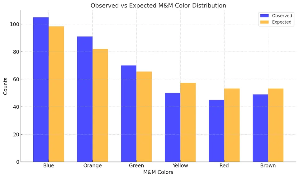
Analysis Results:
- Chi-square statistic: 4.32
- p-value: 0.5045
- Critical value: 11.07
- Decision: Fail to reject the null hypothesis.
Based on this sample, there is insufficient evidence to conclude that the M&M color distribution differs from the specified 2008 distribution.
2. Testing Homogeneity
A chi-square test of homogeneity compares the distribution of a categorical variable across several populations or groups.
Hypotheses
- Null Hypothesis ($H_0$): The categorical variable has the same distribution in all populations or groups.
- Alternative Hypothesis ($H_A$): At least one population or group has a different distribution.
Example: Titanic Survival by Ticket Class
Suppose we want to test whether survival rates are the same across Titanic ticket classes.
Data Summary:
| Survived | Died | Total | |
|---|---|---|---|
| First Class | 203 | 122 | 325 |
| Second Class | 118 | 167 | 285 |
| Third Class | 178 | 528 | 706 |
| Crew | 212 | 673 | 885 |
| Total | 711 | 1,490 | 2,201 |
The null hypothesis is that the survival distribution is the same across all four groups.
Calculating Expected Counts
If the survival distribution were the same across groups, the expected count in cell $(i,j)$ would be:
For First Class survivors:
The observed number of First Class survivors is 203, which is much larger than this expected count.
Computing the Chi-Square Statistic
The statistic is:
Here:
- $r=4$ groups,
- $c=2$ survival outcomes.
Summing across all eight cells gives:
Degrees of Freedom
For a contingency table:
Therefore:
Decision Rule
At:
the critical value for $df=3$ is approximately:
Because:
we reject the null hypothesis.
The p-value is also extremely small:
Interpretation
The data provide very strong evidence that survival rates were not the same across the four Titanic groups.
In other words, survival and ticket-class group are associated in these data. The chi-square test does not explain why the groups differ.
Visualization
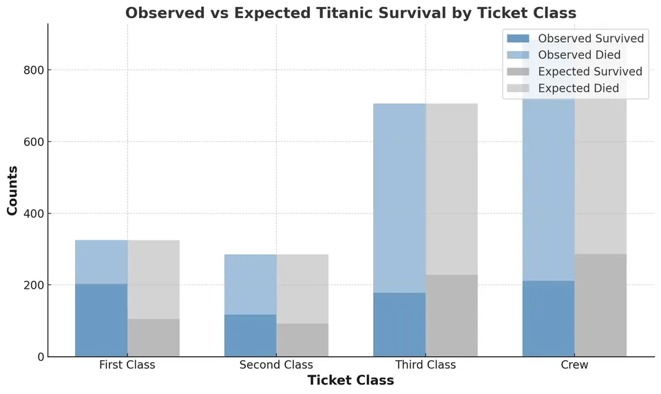
Analysis Results:
- Chi-square statistic: 190.40
- p-value: approximately $5.0\times10^{-41}$
- Critical value: 7.81
- Decision: Reject the null hypothesis.
The data provide strong evidence that survival rates differed among First Class, Second Class, Third Class, and Crew.
3. Testing Independence
A chi-square test of independence examines whether two categorical variables are associated within a population.
Hypotheses
- The null hypothesis ($H_0$) states that the two categorical variables are independent.
- The alternative hypothesis ($H_A$) states that the variables are associated.
If two variables are independent, knowing the value of one does not change the distribution of the other.
Example: Gender and Voting Preference
Suppose we survey individuals to investigate whether gender is associated with voting preference.
Data Summary:
| Liberal | Conservative | Total | |
|---|---|---|---|
| Male | 40 | 60 | 100 |
| Female | 70 | 30 | 100 |
| Total | 110 | 90 | 200 |
If the variables were independent, both gender groups would have the same voting-preference distribution apart from sampling variation.
Calculating Expected Counts
Under independence:
For Male/Liberal:
The expected counts are therefore:
| Liberal | Conservative | |
|---|---|---|
| Male | 55 | 45 |
| Female | 55 | 45 |
Computing the Chi-Square Statistic
The Pearson chi-square statistic is:
For these data:
Degrees of Freedom
Yates' Correction for Continuity (Optional)
For a $2\times2$ table, Yates' continuity correction may be applied:
For these data:
with:
Without the correction, the Pearson test gives:
Both lead to the same conclusion.
Decision Rule
At:
the chi-square critical value with one degree of freedom is approximately:
Using either statistic:
so we reject $H_0$.
Interpretation
The data provide strong evidence of an association between gender and voting preference in the sampled population.
This indicates association, not necessarily causation.
Visualization
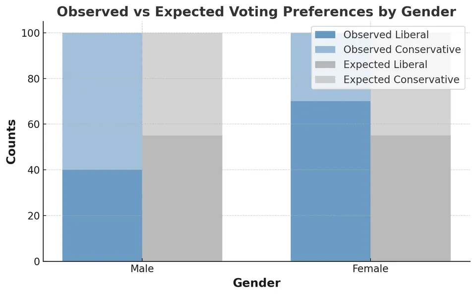
Analysis Results:
Using Yates' continuity correction:
- Chi-square statistic: 16.99
- p-value: $3.76\times10^{-5}$
- Critical value: 3.84
- Decision: Reject the null hypothesis.
There is strong evidence of an association between gender and voting preference in the observed data.
Comparing Homogeneity and Independence Tests
The chi-square tests of homogeneity and independence use the same test statistic and expected-count formula. Their main difference lies in the research question and how the data are collected.
Chi-Square Test of Homogeneity
- The objective is to determine whether several populations or groups have the same distribution of a categorical variable.
- The data structure typically involves separate samples or predefined groups.
- An example is comparing the distribution of M&M colors across different product types, such as milk chocolate, peanut, and caramel.
Chi-Square Test of Independence
- The objective is to determine whether two categorical variables are associated within a population.
- The data structure typically consists of one sample in which each observation is classified by both variables.
- An example is examining the relationship between gender and voting preference in a survey.
Key Differences
The population structure differs:
- In a homogeneity test, distributions are compared across populations or groups.
- In an independence test, two variables are studied within one population.
The research question also differs:
- A homogeneity test asks whether the distribution of a categorical variable is the same across groups.
- An independence test asks whether two categorical variables are associated.
The calculations are otherwise essentially the same once the contingency table has been constructed.
Assumptions and Conditions
For chi-square tests to be valid, several conditions should be checked:
-
The data are counts. The test is applied to observed frequencies in categories.
-
Categories are mutually exclusive. Each observation contributes to one relevant category or table cell.
-
Observations are independent. One observation should not determine or duplicate another.
-
The sampling design should support the intended inference.
-
Expected counts should not be too small. A common rule of thumb is that expected counts should generally be at least 5.
These conditions help ensure that the chi-square distribution provides a reasonable approximation to the sampling distribution of the test statistic.
Practical Application Steps
- State the hypotheses and identify the appropriate chi-square test.
- Organize the observed counts into a frequency table or contingency table.
- Calculate the expected counts under the null hypothesis.
- Check the assumptions, especially independence and expected counts.
- Compute the chi-square statistic:
- Determine the degrees of freedom.
- Find the p-value or critical value using the appropriate chi-square distribution.
- Make a decision by comparing the p-value with $\alpha$, or the test statistic with the critical value.
- Interpret the result in the context of the research question.
A chi-square test tells us whether the observed differences are larger than would reasonably be expected under the null hypothesis. It does not, by itself, explain why an association exists or establish causation.