Spatial Data, Support, and Distance
Spatial analysis begins before any spatial statistic is calculated.
Before using Moran's $I$, fitting a variogram, running kriging, or analyzing a point pattern, we first need to decide what the spatial observations actually represent.
The most important questions are:
- What is the spatial object?
- What coordinate reference system is being used?
- What spatial support does each observation represent?
- What study boundary defines what could have been observed?
- What notion of distance is scientifically meaningful?
- At what spatial scale should the conclusion be interpreted?
These choices affect every method that follows.
Learning objectives
After this chapter, you should be able to:
- distinguish areal data, point-referenced data, and point patterns;
- explain why longitude/latitude coordinates are not ordinary Cartesian coordinates;
- calculate and interpret a great-circle distance;
- explain what spatial support means;
- explain why changing support changes variance and apparent spatial smoothness;
- distinguish the scale and zoning forms of the modifiable areal unit problem;
- explain why distance is a scientific modeling decision;
- distinguish Euclidean, network, travel-time, geodesic, and resistance distance;
- explain why study boundaries matter;
- write down the spatial assumptions that should be documented before modeling.
Three common spatial data objects
Many spatial analyses go wrong because the analyst starts with a technique instead of identifying the data-generating object.
Three spatial data objects recur throughout spatial statistics.
Areal or lattice data
For areal data, one value is attached to each region or cell.
Write
$$ y_i \quad\text{for region }A_i. $$
Examples include:
- unemployment rate by county;
- disease incidence by district;
- crop yield by field;
- average income by census tract;
- vegetation index by raster cell.
The region itself is part of what is observed.
A county unemployment rate is not a point measurement taken at the county centroid. It summarizes people or households distributed across the county.
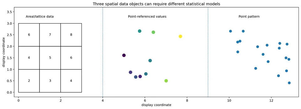
Point-referenced measurements
For point-referenced data, a quantity is measured at sampling locations.
Write
$$ Z(s_i), \qquad s_i\in\mathbb R^2. $$
Examples include:
- soil pH measured at sampling sites;
- rainfall measured at gauges;
- groundwater level measured at wells;
- air pollution measured at monitoring stations.
The sampling locations are usually treated as known design locations.
The spatially varying quantity
$$ Z(s) $$
is the random object of interest.
This is the setting used in geostatistics and kriging.
Point patterns
For point-pattern data, the locations themselves are the observed outcome.
Write
$$ \{s_1,\ldots,s_N\}. $$
Examples include:
- tree stems;
- earthquake epicenters;
- disease cases;
- animal nests;
- retail stores;
- crime incidents.
Here both the number of events and their locations can be random.
This is fundamentally different from measuring a value at a fixed sampling location.
Why the distinction matters
Suppose we have 40 geographic coordinates.
Those 40 coordinates could represent:
- 40 fixed air-quality stations;
- 40 tree locations;
- 40 district centroids.
They may look identical in a scatterplot, but they represent different statistical objects.
For the air-quality stations, we may model
$$ Z(s). $$
For the trees, we model the point process generating locations.
For districts, we model region-level outcomes and neighborhood relationships.
The appropriate method depends on what the coordinates represent.
Coordinate reference systems
Coordinates have meaning only relative to a coordinate reference system (CRS).
A CRS specifies how positions on or near the Earth are represented numerically.
Two broad cases are important:
- geographic coordinates;
- projected coordinates.
Geographic coordinates: longitude and latitude
Longitude and latitude are angular coordinates.
They are usually measured in degrees.
A coordinate such as
$$ (13.4^\circ E, 52.5^\circ N) $$
does not mean 13.4 km east and 52.5 km north.
A naive Euclidean calculation in degree space is
$$ d_{\text{deg}} = \sqrt{ (\Delta\text{lon})^2+ (\Delta\text{lat})^2 }. $$
The result is in degrees, not meters or kilometers.
Why one degree is not one fixed distance
One degree of latitude corresponds to roughly the same north-south distance over much of the Earth.
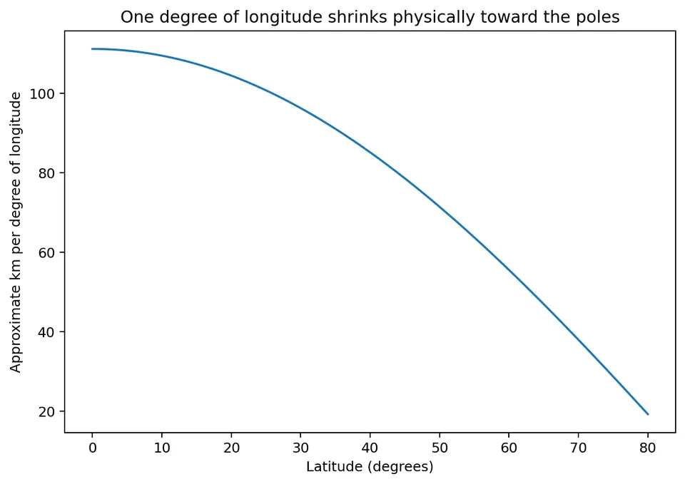
One degree of longitude does not correspond to a fixed physical distance.
Its east-west length decreases as latitude increases.
Approximately,
$$ \text{longitude distance} \propto \cos(\phi), $$
where $\phi$ is latitude.
At the equator,
$$ \cos(0^\circ)=1. $$
At latitude
$$ 60^\circ, $$
$$ \cos(60^\circ)=0.5. $$
So one degree of longitude near $60^\circ$ latitude is roughly half the east-west distance of one degree at the equator.
Numerical example: one degree of longitude
The Earth's mean radius is approximately
$$ R=6371\text{ km}. $$
The length of one degree along a great circle is approximately
$$ \frac{2\pi R}{360}. $$
Substitute:
$$ \frac{2\pi(6371)}{360} \approx111.2\text{ km}. $$
At latitude $\phi$, one degree of longitude is approximately
$$ 111.2\cos(\phi)\text{ km}. $$
At the equator
$$ 111.2\cos(0^\circ) = 111.2\text{ km}. $$
At $45^\circ$
$$ 111.2\cos(45^\circ) \approx 111.2(0.7071) $$
$$ \approx78.6\text{ km}. $$
At $60^\circ$
$$ 111.2\cos(60^\circ) = 111.2(0.5) $$
$$ \boxed{ 55.6\text{ km} }. $$
The same one-degree longitude difference therefore represents very different physical distances.
Great-circle distance
For large geographic extents, distance along the Earth's surface is often more appropriate than planar Euclidean distance.
A common formula for great-circle distance is the haversine formula.
For two points with latitude/longitude
$$ (\phi_1,\lambda_1) $$
and
$$ (\phi_2,\lambda_2), $$
in radians, define
$$ \Delta\phi=\phi_2-\phi_1, \qquad \Delta\lambda=\lambda_2-\lambda_1. $$
Then
$$ a = \sin^2\left(\frac{\Delta\phi}{2}\right) + \cos(\phi_1)\cos(\phi_2) \sin^2\left(\frac{\Delta\lambda}{2}\right). $$
The central angle is
$$ c = 2\arctan2(\sqrt a,\sqrt{1-a}). $$
The great-circle distance is
$$ \boxed{ d=Rc }. $$
This treats the Earth as a sphere of radius $R$. Geodesic distance on an ellipsoid (such as WGS84) can differ from the spherical value by a few tenths of a percent, which matters only for high-accuracy work.
Worked great-circle example
Consider two locations on the equator:
$$ (0^\circ,0^\circ) $$
and
$$ (0^\circ,1^\circ). $$
Then
$$ \Delta\phi=0 $$
and
$$ \Delta\lambda=1^\circ = \frac{\pi}{180} \text{ radians}. $$
So
$$ a = \sin^2\left( \frac{\pi/180}{2} \right). $$
This gives
$$ c \approx0.0174533. $$
With
$$ R=6371\text{ km}, $$
$$ d = 6371(0.0174533) $$
$$ \boxed{ d\approx111.2\text{ km} }. $$
The same one-degree longitude difference at $60^\circ$ latitude is only about 55.6 km.
Projected coordinate systems
A projected CRS maps part of the curved Earth onto a plane.
Coordinates are then often expressed in linear units such as:
- meters;
- feet.
For a suitable local projection, Euclidean distance
$$ d = \sqrt{ (x_2-x_1)^2+ (y_2-y_1)^2 } $$
can be interpreted directly in meters.
Example
Suppose projected coordinates are
$$ s_1=(500000,5700000) $$
and
$$ s_2=(500300,5700400), $$
in meters.
Then
$$ \Delta x=300, \qquad \Delta y=400. $$
Therefore
$$ d = \sqrt{300^2+400^2} = \sqrt{90000+160000} = \sqrt{250000} $$
$$ \boxed{ d=500\text{ m} }. $$
This is the familiar 3-4-5 triangle scaled by 100.
Projection choice still matters
No projection can preserve every spatial property simultaneously.
Different projections may preserve different properties better:
- area;
- shape;
- direction;
- distance over limited regions.
A projection appropriate for a local city-scale analysis may be poor for a continent-wide study.
The important question is therefore not:
Is the data projected?
It is:
Is the projection suitable for the region and measurement being analyzed?
Spatial support
Spatial support is the spatial region over which a measurement is defined, measured, or averaged.
Examples:
- a sensor reading approximates point support;
- a satellite pixel summarizes an area;
- a county rate summarizes a polygon;
- a soil composite sample may summarize several subsamples over a field plot.
Support describes what a single observed value represents spatially.
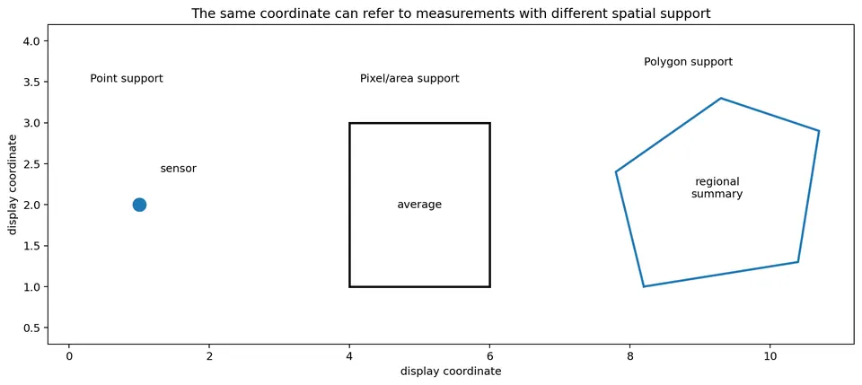
Point support versus area support
Suppose temperature is measured in two ways.
Point-support measurement
A weather station reports
$$ 22.4^\circ C. $$
That reading describes conditions near the sensor location.
Area-support measurement
A satellite product reports average temperature over a
$$ 1\text{ km}\times1\text{ km} $$
pixel.
That value averages conditions over an entire square kilometer.
Even if the pixel center is exactly at the station coordinate, the two observations do not have the same spatial support.
A matching centroid does not make the measurements equivalent.
Why support changes variability
Averaging over larger regions tends to smooth local variation.
Suppose four point-level values inside a block are
$$ 8,\ 10,\ 14,\ 16. $$
Their mean is
$$ \bar x = \frac{8+10+14+16}{4} = 12. $$
If many small-scale fluctuations occur inside regions and only region averages are retained, the resulting area-level data will usually vary less than the original point-level data.
This is called a change-of-support effect.
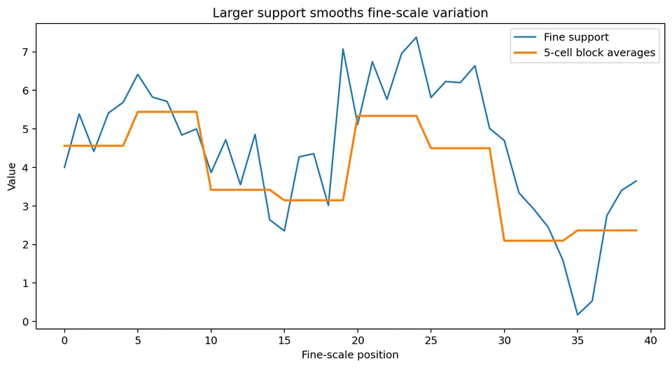
Numerical aggregation example
Suppose eight fine-scale values are
$$ 2,\ 4,\ 6,\ 8,\ 12,\ 14,\ 16,\ 18. $$
Their mean is
$$ 10. $$
The population variance is
$$ \frac{ (2-10)^2+ (4-10)^2+ (6-10)^2+ (8-10)^2+ (12-10)^2+ (14-10)^2+ (16-10)^2+ (18-10)^2 }{8}. $$
The squared deviations are
$$ 64,\ 36,\ 16,\ 4,\ 4,\ 16,\ 36,\ 64. $$
Their sum is
$$ 240. $$
So the fine-scale variance is
$$ \frac{240}{8} = 30. $$
Now aggregate neighboring pairs:
$$ (2,4)\rightarrow3, $$
$$ (6,8)\rightarrow7, $$
$$ (12,14)\rightarrow13, $$
$$ (16,18)\rightarrow17. $$
The four block means are
$$ 3,\ 7,\ 13,\ 17. $$
Their mean is still
$$ 10. $$
Their squared deviations are
$$ 49,\ 9,\ 9,\ 49. $$
The variance is
$$ \frac{116}{4} = 29. $$
The total variance splits into the variance of the block means plus the average within-block variance:
$$ 30 = 29 + 1, $$
because each pair has within-block variance $1$. Aggregation removes only the within-block part.
This small example shows some smoothing, although the amount depends on how the values are arranged. Here neighboring values are very similar, so little variance is lost.
In spatial fields with strong high-frequency variation, aggregation can reduce variance much more dramatically.
Support can change correlation
Suppose two fine-scale variables are noisy:
$$ X(s) $$
and
$$ Y(s). $$
At point level, measurement noise may weaken their observed correlation.
If both variables are averaged over larger regions, some small-scale noise may cancel.
The area-level correlation can therefore be larger than the point-level correlation.
The reverse can also happen.
This is one reason area-level correlations cannot automatically be interpreted as individual-level relationships.
The modifiable areal unit problem
For areal data, statistical results can depend on how space is divided into regions.
This is the modifiable areal unit problem (MAUP).
It has two related forms:
- scale effect;
- zoning effect.
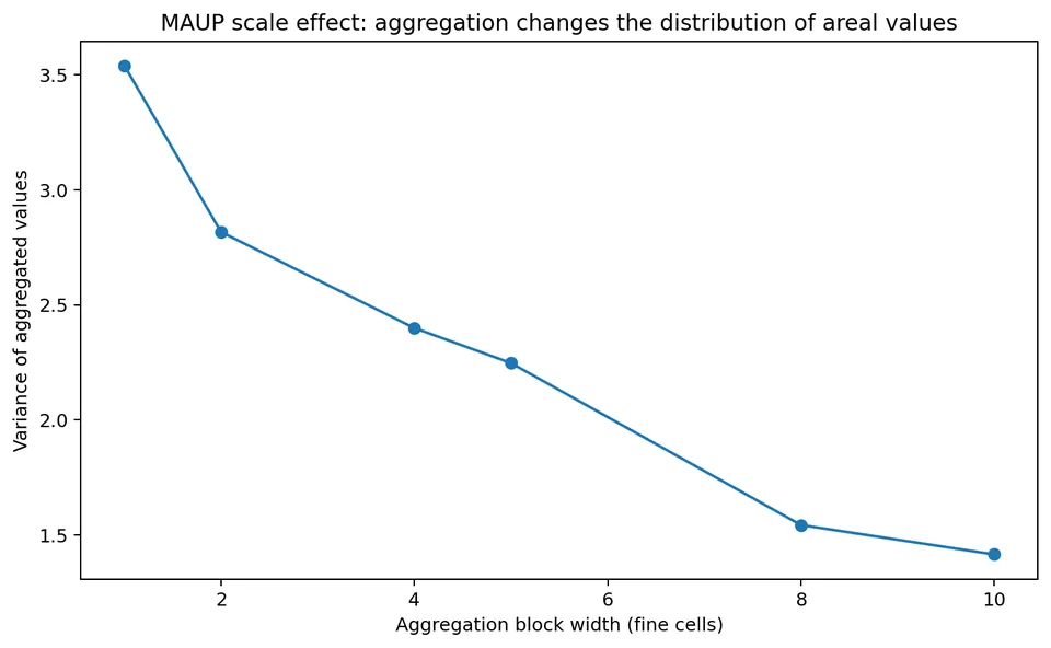
MAUP scale effect
The scale effect occurs when small regions are aggregated into larger ones.
For example:
- census blocks;
- census tracts;
- districts;
- provinces.
The same underlying spatial field can produce different:
- means;
- variances;
- correlations;
- regression slopes;
- cluster statistics
at different aggregation levels.
Numerical scale-effect example
Suppose six small regions have values
$$ 2,\ 3,\ 4,\ 8,\ 9,\ 10. $$
The mean is
$$ 6. $$
Now combine them into three larger regions:
$$ (2,3)\rightarrow2.5, $$
$$ (4,8)\rightarrow6, $$
$$ (9,10)\rightarrow9.5. $$
The larger-unit data are
$$ 2.5,\ 6,\ 9.5. $$
They retain the same broad gradient, but with fewer observations and smoother values.
Any statistic based on local variation or adjacency can change because:
- the number of units changed;
- the values changed;
- the neighborhood graph changed.
The statistic now describes the aggregated regions rather than the original six units.
MAUP zoning effect
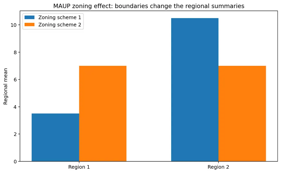
The zoning effect occurs when boundaries change while the number of regions remains similar.
Imagine four fine-scale cells with values
$$ 2,\ 4,\ 8,\ 10. $$
One zoning scheme could group:
$$ (2,4) \quad\text{and}\quad (8,10), $$
producing regional means
$$ 3,\ 9. $$
Another scheme could group:
$$ (2,8) \quad\text{and}\quad (4,10), $$
producing
$$ 5,\ 7. $$
The same fine-scale data can therefore produce very different apparent regional contrasts.
Why MAUP is not just a plotting issue
Suppose a regression coefficient is estimated using district-level data.
If district boundaries are redrawn, both:
- predictor averages;
- outcome averages
can change.
The fitted coefficient may change even though the underlying individuals or fine-scale values have not changed.
Conclusions should therefore state the spatial unit of analysis explicitly.
A statement such as
income is strongly associated with disease
is incomplete if the analysis was actually conducted on county averages.
A better statement is
county-level average income is associated with county-level disease rate under the chosen county geography.
Distance is a modeling choice
The shortest straight-line distance is not always the scientifically relevant distance.
Euclidean distance is
$$ d_{ij} = \sqrt{ (x_i-x_j)^2+ (y_i-y_j)^2 }. $$
It is appropriate when straight-line spatial separation is scientifically meaningful.
Many processes, however, do not operate along straight-line paths.
Road-network distance
Suppose two houses lie on opposite sides of a river.
Their Euclidean distance may be only
$$ 500\text{ m}. $$
If the nearest bridge is several kilometers away, road distance may be
$$ 6\text{ km}. $$
For ambulance response, shopping access, or commuting, the 500 m Euclidean distance may be misleading.
Travel-time distance
Two locations can be the same road distance apart but have different travel times.
For example:
- 10 km along a motorway;
- 10 km through a dense city center.
If the scientific mechanism depends on human movement, travel time may be more meaningful than physical distance.
River-network distance
For aquatic organisms or pollutants, movement may follow a river network.
Two sampling sites can be physically close in straight-line distance but belong to different tributaries.
Their hydrological connection may be weak or nonexistent.
River-network distance can therefore be more meaningful than Euclidean distance for such processes.
Ecological resistance distance
Animals, seeds, or genes may move more easily through some land-cover types than others.
A resistance surface assigns movement cost to the landscape.
Movement through forest might have low resistance while highways or steep terrain have high resistance.
The resulting effective distance can be much larger than the straight-line distance.
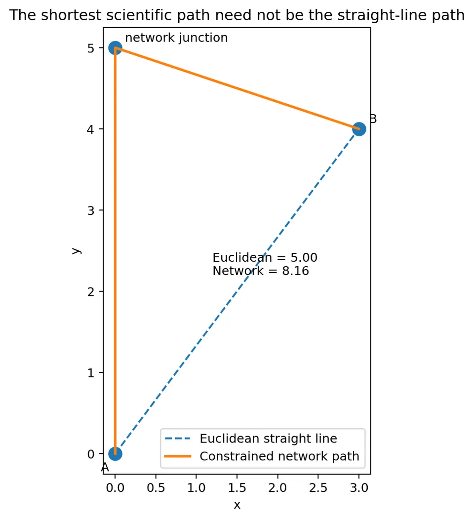
Worked network-distance example
Suppose locations A and B have coordinates
$$ A=(0,0), \qquad B=(3,4). $$
Their Euclidean distance is
$$ \sqrt{3^2+4^2} = 5. $$
But suppose travel must follow a road from A to C to B.
If
$$ d(A,C)=4 $$
and
$$ d(C,B)=5, $$
then network distance is
$$ 4+5 = 9. $$
Thus:
$$ d_{\text{Euclidean}}=5, $$
while
$$ d_{\text{network}}=9. $$
The appropriate distance depends on the process being modeled.
Distance affects spatial weights
Suppose a spatial weights matrix defines neighbors using
$$ d_{ij}\le5\text{ km}. $$
Changing from Euclidean to road-network distance may change whether two locations satisfy the threshold.
That changes:
- the weights matrix;
- Moran's $I$;
- local cluster categories;
- spatial regression structure.
Distance choice therefore propagates into later statistics.
Distance affects geostatistical covariance
A variogram model may use
$$ \gamma(h) $$
where $h$ is separation distance.
If the wrong distance metric is used, the estimated range and covariance structure may be misleading.
For example, two stream sites separated by 1 km Euclidean distance but 12 km along the stream network should not necessarily be treated as strongly related.
Distance affects validation design
Spatial validation often groups observations into blocks.
If blocks are defined using straight-line distance while the scientific process follows travel corridors or rivers, the validation design may not represent the intended transfer problem.
Distance is therefore more than a preprocessing choice.
It affects the scientific question being evaluated.
Directional and anisotropic distance
Some processes propagate more strongly in one direction than another.
Examples include:
- wind-driven pollution;
- groundwater flow;
- ocean currents;
- geological structures.
An anisotropic distance can stretch one direction relative to another.
A simple example is
$$ d_A = \sqrt{ \left(\frac{\Delta x}{a_x}\right)^2 + \left(\frac{\Delta y}{a_y}\right)^2 }. $$
If
$$ a_x>a_y, $$
then separation in the $x$ direction is treated as effectively shorter than the same physical separation in $y$.
This represents longer spatial dependence along the $x$ direction.
Study-region boundaries
Every spatial study has a domain or observation window.
For areal data, this may be a set of administrative units.
For geostatistics, it may be the sampled landscape.
For a point process, it is the region in which events could have been observed.
The boundary is part of both the data-generating process and the observation process.
Why boundaries matter
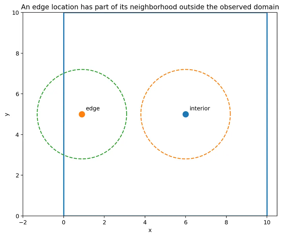
Consider a point near the edge of a study region.
It has less observed surrounding area than an interior point.
A point-process neighborhood of radius $r$ may extend outside the observation window.
Similarly, a location near a national border may have relevant neighbors across the border that are absent from the dataset.
Ignoring boundaries can create:
- missing neighbors;
- biased pair counts;
- artificial edge effects;
- misleading spatial weights.
Administrative boundaries versus process boundaries
A dataset may end at an administrative boundary even when the physical process does not.
Examples:
- air pollution crosses state borders;
- groundwater crosses county boundaries;
- commuter flows cross municipal boundaries;
- wildlife moves across park boundaries.
The data boundary and the scientific process boundary are not necessarily the same.
This should be documented explicitly.
Support mismatch
Two datasets may cover the same geographic area but have incompatible support.
Example:
- air pollution: 1 km raster cells;
- health outcome: county-level rate;
- income: census-tract average.
A naive merge based only on centroid proximity can combine incompatible spatial supports.
Before regression or correlation, determine which transformation is scientifically appropriate.
Possible approaches include:
- area-weighted aggregation;
- population-weighted aggregation;
- point-to-area integration;
- explicit change-of-support models.
Example: area-weighted aggregation
Suppose a county overlaps two raster cells.
Cell 1 has value
$$ 10 $$
and contributes 70% of the county area.
Cell 2 has value
$$ 20 $$
and contributes 30%.
An area-weighted county average is
$$ 0.7(10)+0.3(20). $$
Therefore
$$ 7+6 = \boxed{ 13 }. $$
A simple unweighted average would be
$$ 15, $$
which gives the two cells equal importance even though their overlap with the county differs greatly.
Area weighting is not always enough
Suppose the raster represents air pollution and the county outcome represents human exposure.
If nearly all people live in the 30% portion of the county associated with the second raster cell, area weighting may poorly represent population exposure.
A population-weighted average might be more appropriate.
This illustrates a general principle:
Aggregation weights should reflect the spatial and scientific support of the target quantity.
Before modeling: a spatial data audit
Before running a spatial method, document the following.
Spatial object
Is the dataset:
- areal/lattice;
- point-referenced;
- a point pattern?
CRS and units
Are coordinates:
- longitude/latitude in degrees;
- projected meters;
- another system?
Support
Does each value represent:
- a point;
- pixel;
- polygon;
- moving window;
- population average?
Boundary
What region defines the study?
Is it:
- physical;
- administrative;
- observational?
Distance or neighborhood
What notion of closeness represents the scientific process?
Intended scale of inference
Does the conclusion apply to:
- individuals;
- pixels;
- neighborhoods;
- districts;
- regions?
A complete worked example
Suppose a researcher wants to study heat and health.
Available data are:
- temperature raster: 1 km pixels;
- hospital admissions: counts by district;
- district population;
- district boundaries in longitude/latitude.
Several decisions must be made before the analysis begins.
identify the spatial objects
Temperature is area-supported raster data.
Hospital admissions are areal counts.
Population is also areal, but may represent residential exposure rather than physical area.
choose a suitable CRS
For local planar calculations, project the district boundaries and raster to an appropriate local CRS.
reconcile support
Aggregate raster temperature to districts.
If health risk relates to where people live, population-weighted temperature may be more relevant than area-weighted temperature.
define neighborhood
For spatial autocorrelation in residual disease risk, adjacency may be scientifically meaningful.
For heat exposure, physical distance might be more meaningful.
interpret results at the correct scale
A district-level association is a district-level ecological result.
It does not automatically describe individual-level risk.
Common mistakes
treating longitude and latitude as Cartesian meters
Degree differences are angular quantities, not linear distances.
assuming any projected CRS is suitable
Projection distortion depends on the region and the intended use.
treating polygon centroids as if observations had point support
The value usually summarizes the entire polygon.
aggregating without considering change of support
Aggregation changes variance and can also change correlation.
ignoring MAUP
Results can depend on both scale and zoning.
assuming Euclidean distance is always scientifically meaningful
Relevant movement may follow roads, rivers, currents, or resistance surfaces.
forgetting the boundary
Missing space outside the study region can bias neighborhood and point-process summaries.
mixing spatial scales in interpretation
A county-level result is not automatically an individual-level result.
Concept map
The correct sequence is:
$$ \text{spatial dataset} $$
$$ \downarrow $$
$$ \text{identify spatial object} $$
$$ \downarrow $$
$$ \text{check CRS and units} $$
$$ \downarrow $$
$$ \text{identify support} $$
$$ \downarrow $$
$$ \text{define study boundary} $$
$$ \downarrow $$
$$ \text{choose scientifically meaningful distance/neighborhood} $$
$$ \downarrow $$
$$ \text{state intended scale of inference} $$
$$ \downarrow $$
$$ \text{only then choose a spatial model or statistic}. $$
The central lesson is:
Spatial coordinates are not enough. Spatial analysis depends on what the observations represent, over what support they are defined, and which geometry matches the scientific process.
Questions students should be able to answer
- What is the difference between point-referenced data and a point pattern?
- Why is an areal value not simply a point located at its centroid?
- Why is Euclidean distance in longitude/latitude degree space problematic?
- Why does one degree of longitude represent different distances at different latitudes?
- When is a projected CRS useful?
- What is spatial support?
- Why does aggregation usually smooth spatial data?
- What is the difference between the MAUP scale effect and zoning effect?
- Why can different zoning systems change a regression result?
- When might road-network distance be preferable to Euclidean distance?
- When might geodesic distance be preferable to projected Euclidean distance?
- Why can a study boundary create missing neighbors?
- Why can area-weighted aggregation be inappropriate for human exposure?
- What should be documented before computing a spatial statistic?