Kriging
Kriging is a method for predicting a spatial variable at unsampled locations using a model of spatial dependence.
Kriging is often introduced as the best linear unbiased predictor (BLUP). The phrase is useful when each part is interpreted carefully:
- linear: the prediction is a weighted sum of observed values;
- unbiased: the weights satisfy constraints implied by the assumed mean model;
- best: among predictors that satisfy those assumptions, kriging minimizes prediction variance;
- predictor: it predicts an unknown spatial quantity.
Kriging is therefore not simply a generic smoother or a distance-weighted average.
The result depends on:
- the assumed mean structure;
- the covariance or variogram model;
- the geometry of the sample locations;
- the prediction target.
Learning objectives
After this chapter, you should be able to:
- explain what kriging is calculating and why;
- assemble an ordinary-kriging system from coordinates and a semivariogram;
- solve for kriging weights;
- calculate a kriging prediction;
- calculate and interpret kriging variance;
- distinguish ordinary, simple, and universal kriging;
- explain why kriging weights are not merely inverse-distance weights;
- explain how nearby observations can be redundant;
- explain when kriging interpolates exactly and when it may smooth;
- perform and interpret leave-one-out cross-validation;
- explain why low kriging variance does not prove that the model is correct.
The prediction problem
Suppose we have observations
$$ Z(s_1),Z(s_2),\ldots,Z(s_n) $$
at sampled spatial locations
$$ s_1,s_2,\ldots,s_n. $$
We want to predict the field at an unsampled location
$$ s_0. $$
Kriging uses a linear predictor
$$ \hat Z(s_0) = \sum_{i=1}^n\lambda_i Z(s_i). $$
The numbers
$$ \lambda_1,\lambda_2,\ldots,\lambda_n $$
are the kriging weights.
What is being calculated?
Kriging calculates weights that satisfy the mean-model constraints while minimizing the variance of the prediction error.
The prediction error is
$$ Z(s_0)-\hat Z(s_0). $$
Kriging chooses the weights to minimize
$$ \mathrm{Var} \left[ Z(s_0)-\hat Z(s_0) \right] $$
under the assumed spatial model.
Why not just use the nearest observation?
The nearest observation may be informative, but it is not necessarily sufficient.
Several observations may jointly contain information about the target.
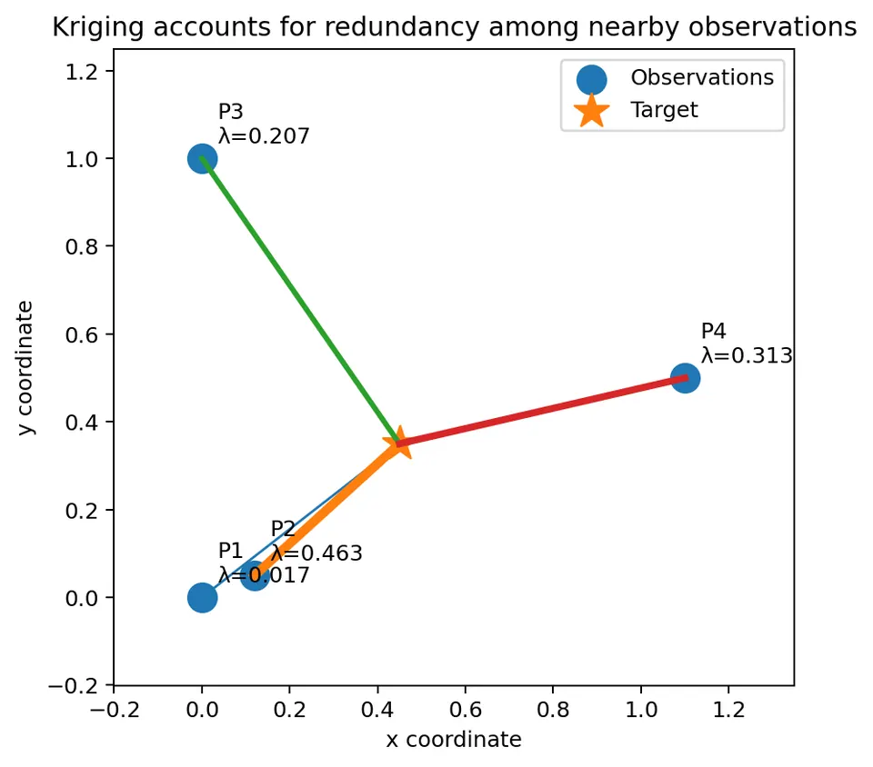
Kriging also accounts for redundancy among nearby observations. Two points almost on top of each other do not provide twice as much independent information as one point.
This is one reason kriging differs from simple distance-based weighting.
Ordinary kriging
Ordinary kriging assumes that the mean is:
- unknown;
- constant over the local spatial domain.
Write
$$ E[Z(s)]=m, $$
where the constant $m$ is unknown.
The ordinary-kriging predictor is
$$ \hat Z(s_0) = \sum_{i=1}^n\lambda_i Z(s_i). $$
For this predictor to be unbiased for any unknown constant mean, the weights must satisfy
$$ \sum_{i=1}^n\lambda_i=1. $$
Why must the weights sum to 1?
Take expectations:
$$ E[\hat Z(s_0)] = E\left[ \sum_i\lambda_i Z(s_i) \right]. $$
Because expectation is linear,
$$ E[\hat Z(s_0)] = \sum_i\lambda_i E[Z(s_i)]. $$
Under the ordinary-kriging mean assumption,
$$ E[Z(s_i)]=m. $$
Therefore
$$ E[\hat Z(s_0)] = m\sum_i\lambda_i. $$
For the predictor to have expected value $m$,
$$ m\sum_i\lambda_i=m. $$
Thus
$$ \boxed{ \sum_i\lambda_i=1 }. $$
The sum-to-one constraint is therefore not arbitrary. It preserves an unknown constant mean.
Ordinary kriging with a semivariogram
Using a valid semivariogram $\gamma$, the ordinary-kriging system is
$$ \begin{bmatrix} \Gamma & \mathbf{1}\\ \mathbf{1}^{\top} & 0 \end{bmatrix} \begin{bmatrix} \lambda\\ \mu \end{bmatrix} = \begin{bmatrix} \gamma_0\\ 1 \end{bmatrix}, $$
where
$$ \Gamma_{ij} = \gamma(s_i-s_j) $$
and
$$ (\gamma_0)_i = \gamma(s_i-s_0). $$
Here:
- $\Gamma$ contains semivariogram values among the observations;
- $\gamma_0$ contains semivariogram values between each observation and the target;
- $\lambda$ contains the unknown kriging weights;
- $\mu$ is a Lagrange multiplier that enforces the sum-to-one constraint.
With this sign convention,
$$ \sigma_K^2(s_0) = \lambda^\top\gamma_0+\mu. $$
Some texts use the opposite sign for the multiplier. Either convention is valid as long as the kriging system and variance formula are consistent.
Fully worked ordinary-kriging example
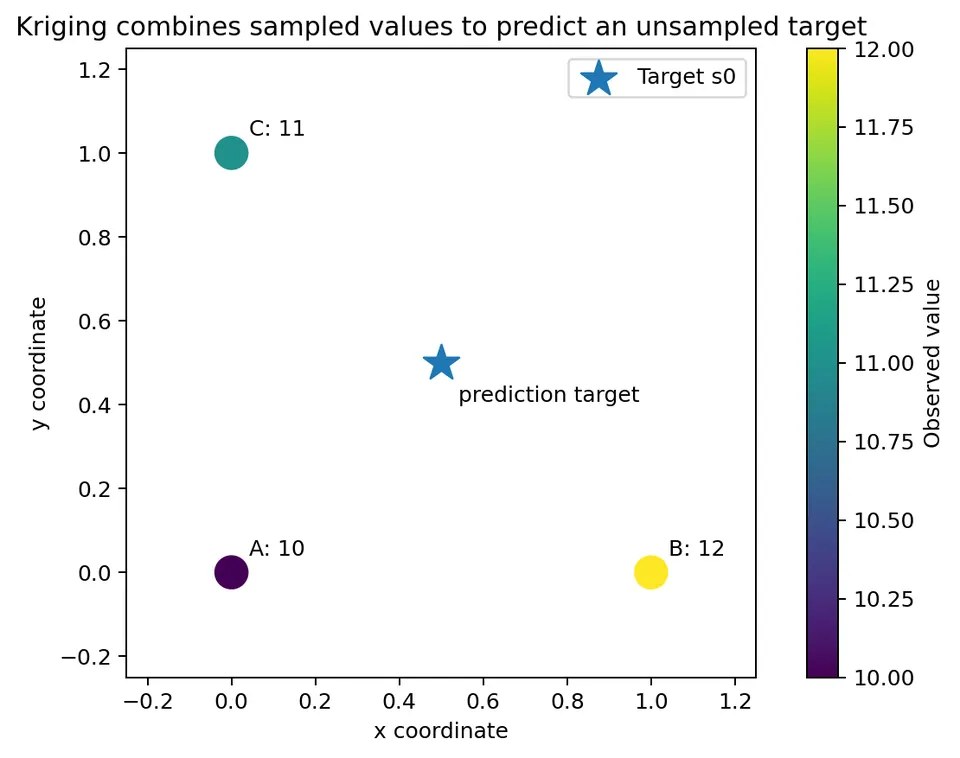
Consider three sampled points:
| Point | Coordinate | Observed value |
|---|---|---|
| A | $(0,0)$ | 10 |
| B | $(1,0)$ | 12 |
| C | $(0,1)$ | 11 |
We want to predict at
$$ s_0=(0.5,0.5). $$
Use the exponential semivariogram
$$ \gamma(h) = 0.2 + 2.8\left(1-e^{-h/1.5}\right), \qquad h>0, $$
with
$$ \gamma(0)=0. $$
This example is small enough to work through by hand.
calculate distances among observations
The observation coordinates are
$$ A=(0,0), \qquad B=(1,0), \qquad C=(0,1). $$
Distance A-B:
$$ d_{AB} = \sqrt{(1-0)^2+(0-0)^2} = 1. $$
Distance A-C:
$$ d_{AC} = \sqrt{(0-0)^2+(1-0)^2} = 1. $$
Distance B-C:
$$ d_{BC} = \sqrt{(1-0)^2+(0-1)^2} = \sqrt{2} \approx1.4142. $$
calculate semivariogram values among observations
For distance 1,
$$ \gamma(1) = 0.2 + 2.8\left(1-e^{-1/1.5}\right). $$
Because
$$ e^{-1/1.5} = e^{-0.6667} \approx0.5134, $$
we obtain
$$ \gamma(1) \approx 0.2+2.8(1-0.5134). $$
Thus
$$ \gamma(1) \approx 0.2+2.8(0.4866) $$
$$ \gamma(1) \approx 1.5624. $$
For distance $\sqrt{2}$,
$$ \gamma(\sqrt{2}) = 0.2 + 2.8 \left( 1-e^{-\sqrt{2}/1.5} \right). $$
Numerically,
$$ \gamma(\sqrt{2}) \approx1.9093. $$
The observation-to-observation semivariogram matrix is therefore
$$ \Gamma \approx \begin{bmatrix} 0 & 1.5624 & 1.5624\\ 1.5624 & 0 & 1.9093\\ 1.5624 & 1.9093 & 0 \end{bmatrix}. $$
The diagonal is zero because
$$ \gamma(0)=0. $$
calculate distances from observations to the target
The target is
$$ s_0=(0.5,0.5). $$
Distance from A:
$$ d_{A0} = \sqrt{(0.5-0)^2+(0.5-0)^2} $$
$$ = \sqrt{0.25+0.25} = \sqrt{0.5} \approx0.7071. $$
The same distance occurs from B and C:
$$ d_{B0}=d_{C0}\approx0.7071. $$
Now calculate the semivariogram:
$$ \gamma(0.7071) = 0.2 + 2.8\left( 1-e^{-0.7071/1.5} \right). $$
Numerically,
$$ \gamma(0.7071)\approx1.2524. $$
Thus
$$ \gamma_0 \approx \begin{bmatrix} 1.2524\\ 1.2524\\ 1.2524 \end{bmatrix}. $$
assemble the augmented kriging system
The ordinary-kriging system becomes
$$ \begin{bmatrix} 0 & 1.5624 & 1.5624 & 1\\ 1.5624 & 0 & 1.9093 & 1\\ 1.5624 & 1.9093 & 0 & 1\\ 1 & 1 & 1 & 0 \end{bmatrix} \begin{bmatrix} \lambda_A\\ \lambda_B\\ \lambda_C\\ \mu \end{bmatrix} = \begin{bmatrix} 1.2524\\ 1.2524\\ 1.2524\\ 1 \end{bmatrix}. $$
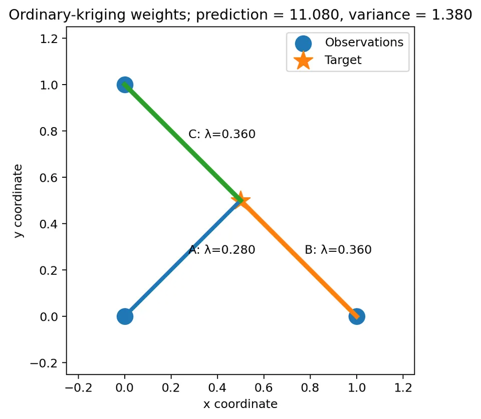
Solving this linear system gives approximately
$$ \lambda_A=0.2801, $$
$$ \lambda_B=0.3600, $$
$$ \lambda_C=0.3600, $$
and
$$ \mu=0.1276. $$
Check the constraint:
$$ 0.2801+0.3600+0.3600 \approx1. $$
So the ordinary-kriging unbiasedness constraint is satisfied.
Calculate the ordinary-kriging prediction
The observations are
$$ z= \begin{bmatrix} 10\\ 12\\ 11 \end{bmatrix}. $$
The prediction is
$$ \hat Z(s_0) = \lambda^\top z. $$
Substitute the numbers:
$$ \hat Z(s_0) = 0.2801(10) + 0.3600(12) + 0.3600(11). $$
Calculate each contribution:
$$ 0.2801(10)=2.801, $$
$$ 0.3600(12)=4.320, $$
$$ 0.3600(11)=3.960. $$
Add them:
$$ \hat Z(s_0) \approx 2.801+4.320+3.960. $$
Therefore
$$ \boxed{ \hat Z(s_0)\approx11.080 }. $$
What does this mean?
Under the assumed constant-mean model and exponential semivariogram, the kriging prediction at $(0.5,0.5)$ is approximately 11.08.
This prediction is conditional on the assumed model.
A different variogram, trend model, or nugget interpretation could produce different weights and a different prediction.
Calculate the ordinary-kriging variance
With the sign convention used above,
$$ \sigma_K^2(s_0) = \lambda^\top\gamma_0+\mu. $$
We have
$$ \lambda = \begin{bmatrix} 0.2801\\ 0.3600\\ 0.3600 \end{bmatrix} $$
and
$$ \gamma_0 = \begin{bmatrix} 1.2524\\ 1.2524\\ 1.2524 \end{bmatrix}. $$
Therefore
$$ \lambda^\top\gamma_0 = 0.2801(1.2524) + 0.3600(1.2524) + 0.3600(1.2524). $$
Because the weights sum to 1,
$$ \lambda^\top\gamma_0 \approx1.2524. $$
Then
$$ \sigma_K^2(s_0) = 1.2524+0.1276 $$
$$ \boxed{ \sigma_K^2(s_0)\approx1.3800 }. $$
The kriging standard deviation is
$$ \sigma_K(s_0) = \sqrt{1.3800} \approx1.175. $$
What is this uncertainty measuring?
The kriging variance measures prediction uncertainty implied by the sampling geometry and the assumed stochastic model.
It reflects:
- how far the target is from data;
- how observations are arranged around the target;
- the covariance or variogram parameters;
- the mean-model constraints.
Once the covariance parameters are treated as fixed, the kriging variance does not directly depend on whether the observed values are 10, 20, or 100.
This often surprises students.
Why kriging weights are not just inverse-distance weights
Suppose a target is near three observations.
Two observations are nearly on top of one another, while a third observation is at a similar target distance but lies in another direction.
A distance-only method may give all three observations similar importance.
Kriging recognizes that the two nearly coincident observations contain highly redundant information.
The weights depend on the full covariance geometry, not only on distance to the target.
Important consequence
The closest observation does not always receive the largest weight.
Kriging weights depend on:
- each observation's relation to the target;
- each observation's relation to every other observation;
- the mean constraint.
This is why kriging needs the full matrix $\Gamma$, or equivalently the full covariance matrix $C$.
Kriging as a spatial prediction surface
In practice, predictions are usually made at many grid locations.
For every grid location $s_0$:
- calculate the distances from the target to all sampled points;
- convert those distances to covariance or semivariogram values;
- solve the kriging system;
- calculate the weighted prediction;
- calculate kriging variance.
Repeating this process creates a prediction surface.
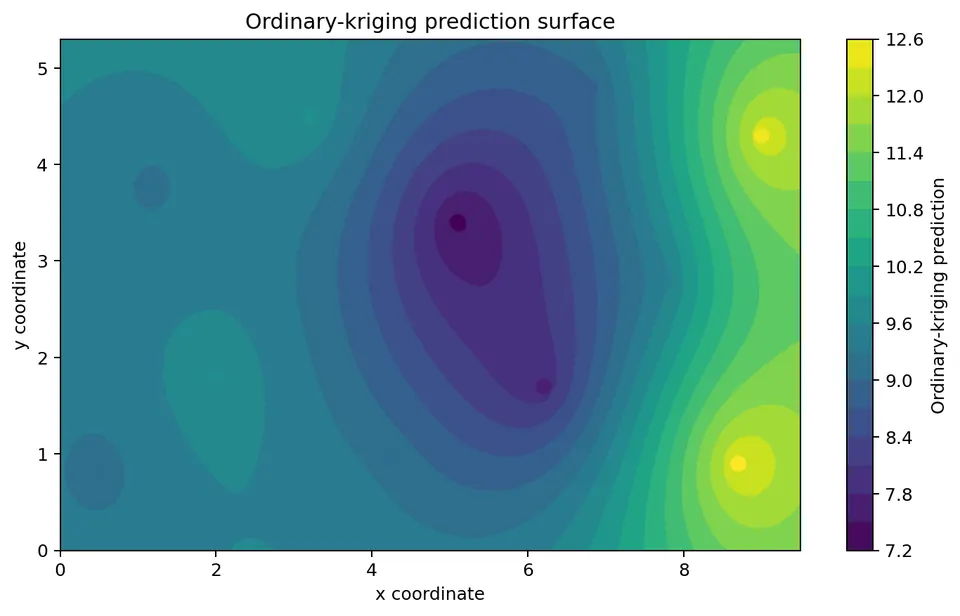
The resulting surface is not merely a visual smoothing of the data. It comes from repeatedly solving the model-based prediction problem.
Kriging variance across space
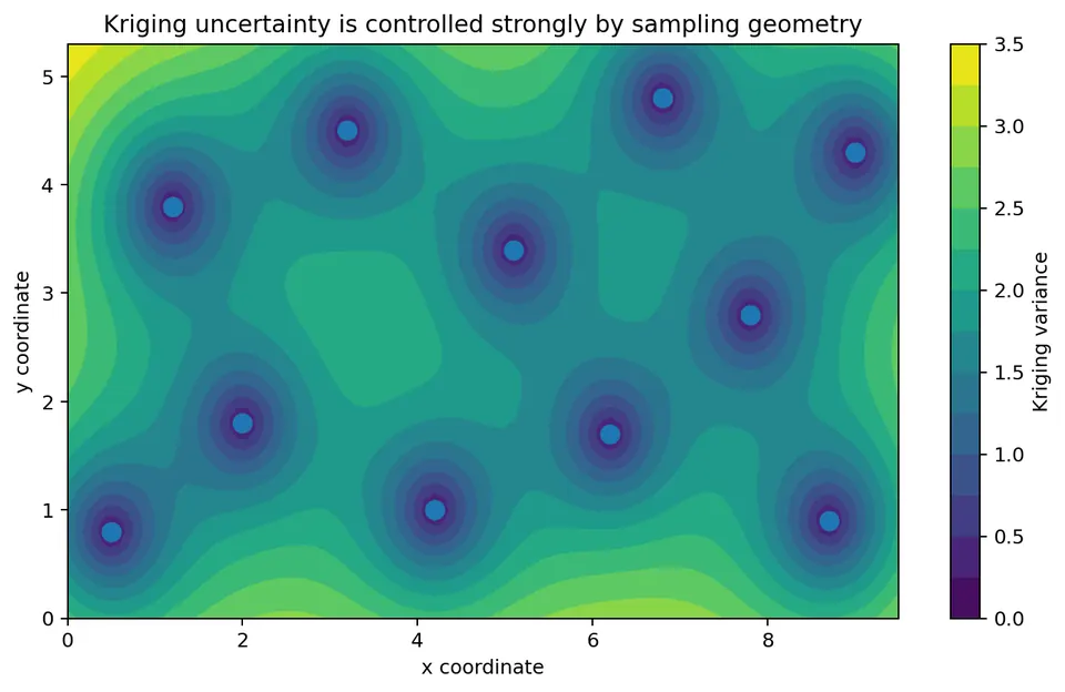
Prediction uncertainty changes with sampling geometry.
Uncertainty is often smaller near sampled locations.
Uncertainty is usually lower inside a dense cluster of observations than in a large unsampled gap.
Outside the convex region covered by data, uncertainty often increases.
A common misconception
A smooth prediction surface does not imply low uncertainty everywhere.
The prediction map and the uncertainty map answer different questions:
- prediction map: "What value does the model predict?"
- variance map: "How uncertain is that prediction under the model?"
Both maps should be examined together.
Simple kriging
Simple kriging assumes the mean is known.
Suppose
$$ E[Z(s)]=m $$
and $m$ is known exactly.
The simple-kriging predictor is
$$ \hat Z(s_0) = m + c_0^\top C^{-1}(z-m\mathbf{1}), $$
where
- $C$ is the covariance matrix among observations;
- $c_0$ is the covariance vector between observations and the target;
- $z$ is the vector of observed values.
The simple-kriging weights are
$$ \lambda=C^{-1}c_0. $$
They do not have to sum to 1.
Why is there no sum-to-one constraint?
Because the known mean is included explicitly:
$$ m + c_0^\top C^{-1}(z-m\mathbf{1}). $$
The model only needs to predict deviations from the known mean.
Simple-kriging numerical example
Suppose the known mean is
$$ m=10. $$
Consider two observations
$$ z= \begin{bmatrix} 12\\ 9 \end{bmatrix}. $$
Their deviations from the mean are
$$ z-m\mathbf{1} = \begin{bmatrix} 2\\ -1 \end{bmatrix}. $$
Suppose the covariance matrix is
$$ C= \begin{bmatrix} 4 & 1.5\\ 1.5 & 4 \end{bmatrix} $$
and covariance with the target is
$$ c_0= \begin{bmatrix} 2.5\\ 1.0 \end{bmatrix}. $$
The weights solve
$$ C\lambda=c_0. $$
The inverse is approximately
$$ C^{-1} \approx \begin{bmatrix} 0.291 & -0.109\\ -0.109 & 0.291 \end{bmatrix}. $$
Thus
$$ \lambda = C^{-1}c_0 \approx \begin{bmatrix} 0.618\\ 0.018 \end{bmatrix}. $$
The simple-kriging prediction is
$$ \hat Z(s_0) = 10 + 0.618(2) + 0.018(-1). $$
Therefore
$$ \hat Z(s_0) \approx 10+1.236-0.018 $$
$$ \boxed{ \hat Z(s_0)\approx11.218 }. $$
Notice that the weights sum to about
$$ 0.618+0.018=0.636, $$
not 1.
That is valid because the known mean accounts for the remaining contribution.
The simple-kriging variance for this example, with $C(0)=4$, is
$$ \sigma_K^2(s_0)=C(0)-c_0^\top\lambda = 4-(2.5\cdot0.618+1.0\cdot0.018)\approx 2.44. $$
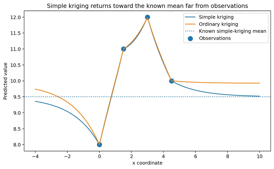
What happens far from all data in simple kriging?
As the target moves far away from every observation,
$$ c_0\rightarrow0. $$
Then
$$ c_0^\top C^{-1}(z-m\mathbf{1}) \rightarrow0. $$
Therefore
$$ \hat Z(s_0)\rightarrow m. $$
Simple kriging therefore returns toward the known mean as the target moves far from the observations.
This is an important conceptual difference between simple and ordinary kriging.
Simple-kriging variance
For a latent process with target variance
$$ C(0), $$
the simple-kriging prediction variance is
$$ \sigma_K^2(s_0) = C(0)-c_0^\top C^{-1}c_0. $$
What is being calculated?
The baseline variance at the target is $C(0)$.
The observations reduce that uncertainty by the amount
$$ c_0^\top C^{-1}c_0. $$
If the target is strongly correlated with informative observations, this reduction is large.
If the target is far from all observations, $c_0$ is close to zero and the prediction variance approaches $C(0)$.
Universal kriging
Ordinary kriging assumes a constant but unknown mean.
That assumption may be inappropriate when the mean changes systematically over space.
Universal kriging models the mean as
$$ m(s)=f(s)^\top\beta. $$
For example,
$$ m(x,y) = \beta_0+\beta_1x+\beta_2y. $$
The vector of basis functions is
$$ f(s) = \begin{bmatrix} 1\\ x\\ y \end{bmatrix}. $$
Universal kriging incorporates this trend structure into the prediction.
Universal-kriging constraints
Let $F$ be the design matrix of trend basis values at the sampled locations.
For a linear coordinate trend,
$$ F = \begin{bmatrix} 1 & x_1 & y_1\\ 1 & x_2 & y_2\\ \vdots & \vdots & \vdots\\ 1 & x_n & y_n \end{bmatrix}. $$
At the target,
$$ f_0 = \begin{bmatrix} 1\\ x_0\\ y_0 \end{bmatrix}. $$
The kriging weights must satisfy
$$ F^\top\lambda=f_0. $$
The covariance-form system is
$$ \begin{bmatrix} C & F\\ F^\top & 0 \end{bmatrix} \begin{bmatrix} \lambda\\ \nu \end{bmatrix} = \begin{bmatrix} c_0\\ f_0 \end{bmatrix}. $$
Why are there multiple constraints?
Ordinary kriging only needs to preserve a constant mean.
Universal kriging may need to preserve:
- an intercept;
- an $x$ trend;
- a $y$ trend;
- elevation effects;
- other covariate-based mean terms.
These additional constraints ensure that the predictor preserves the modeled trend.
Universal-kriging trend example
Suppose the mean is
$$ m(x,y) = 5+0.8x-0.3y. $$
At target
$$ s_0=(4,2), $$
the mean component is
$$ m(4,2) = 5+0.8(4)-0.3(2). $$
Therefore
$$ m(4,2) = 5+3.2-0.6 = 7.6. $$
Universal kriging does not simply return the trend value 7.6.
Instead, it combines:
- the broad trend prediction;
- spatially correlated residual information from nearby observations.
Conceptually,
$$ \text{prediction} = \text{trend contribution} + \text{kriged residual contribution}. $$
This decomposition is closely related to regression kriging.
Ordinary versus universal kriging
Suppose the true field increases strongly from west to east.
If ordinary kriging is applied over a large region, the covariance model may be forced to absorb part of the trend.
This can produce:
- an artificially large range;
- inflated long-distance covariance;
- biased predictions near boundaries;
- misleading uncertainty.
Universal kriging instead assigns the broad trend to the mean model and uses the covariance model for residual spatial dependence.
A useful modeling principle is:
Explain broad deterministic structure with the mean model when possible, and use the covariance model for the remaining spatial dependence.
Does kriging interpolate exactly?
Students often hear:
"Kriging is an exact interpolator."
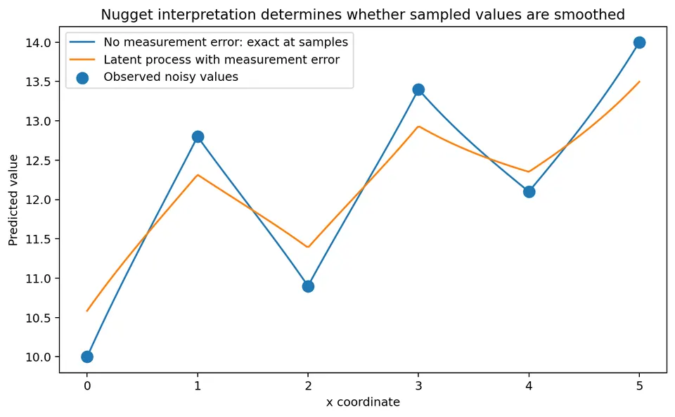
That statement needs qualification because exact interpolation depends on the target and on how the nugget is interpreted.
Whether prediction at a sampled location exactly reproduces the observed value depends on:
- what the nugget means;
- whether the prediction target is the noisy observation or the latent process;
- how the covariance model is constructed.
Nugget as microscale process variation
Suppose the nugget represents real process variation occurring at scales smaller than the sampling spacing.
If the target is the process value at an already observed location, an exact-interpolation convention may be reasonable.
The observed process value is treated as known at that location.
Nugget as measurement error
Suppose instead
$$ Y(s)=X(s)+\epsilon(s), $$
where:
- $X(s)$ is the latent true process;
- $\epsilon(s)$ is independent measurement error.
If the target is $X(s)$, the error-free latent field, then even at a sampled coordinate we do not know the target exactly because the observation contains noise.
A smoother prediction can therefore be appropriate.
Example
Suppose an instrument reports
$$ Y(s)=12.0 $$
but the measurement-error standard deviation is known to be substantial.
The prediction of the latent $X(s)$ can combine:
- the measurement at $s$;
- neighboring measurements;
- the spatial covariance model.
The resulting prediction therefore need not equal exactly 12.0.
Main lesson
The key question is not simply:
"Does kriging interpolate?"
A more useful question is:
"What random quantity are we predicting, and how is the nugget interpreted?"
Kriging uncertainty versus model uncertainty
The kriging variance is calculated conditional on the assumed model.
This distinction is important.
A small kriging variance does not guarantee an accurate prediction if the model is wrong.
Possible model failures include:
- wrong mean structure;
- wrong covariance family;
- badly estimated range;
- ignored anisotropy;
- nonstationarity;
- unmodeled boundaries;
- incorrect nugget interpretation.
It is therefore useful to separate two uncertainty questions:
Conditional kriging uncertainty
If the fitted model were correct, how uncertain is the prediction because of spatial sampling geometry and process variability?
Model uncertainty
How uncertain are we because the fitted model itself may be wrong or poorly estimated?
The standard kriging variance primarily addresses the first of these questions.
Why the kriging variance does not directly depend on observed values
After covariance parameters are fixed, ordinary-kriging weights are obtained from:
- coordinates;
- target location;
- covariance or variogram parameters;
- mean constraints.
The values
$$ z_1,\ldots,z_n $$
do not appear in the weight system.
The values are used only after the weights are found:
$$ \hat Z(s_0)=\lambda^\top z. $$
Therefore two datasets measured at the same coordinates with the same covariance model would have:
- the same kriging weights;
- the same kriging variance;
- different predicted values.
This distinction helps clarify what kriging variance represents.
Negative kriging weights
Kriging weights are not required to lie between 0 and 1.
They can sometimes be negative.
Negative weights can occur because the predictor must balance:
- redundancy among observations;
- mean constraints;
- covariance geometry;
- extrapolation.
A negative weight is not automatically a sign of error.
However, very large positive and negative weights can indicate difficult sampling geometry or model instability and should be investigated.
Cross-validation
A fitted kriging model should be validated.
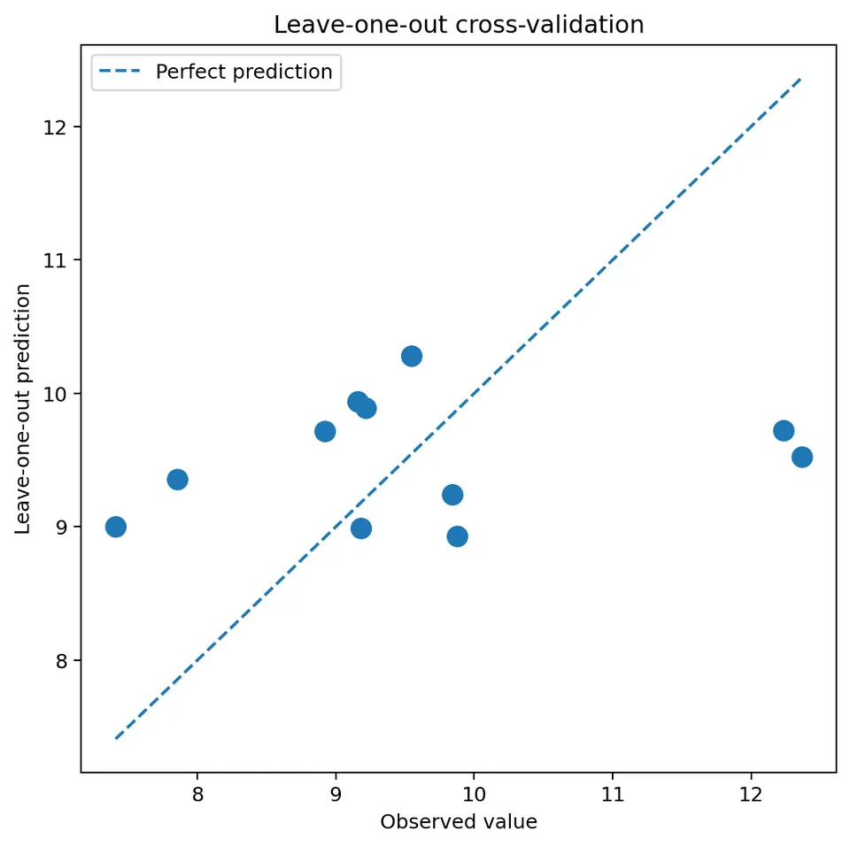
A common diagnostic is leave-one-out cross-validation.
For each observation $i$:
- remove observation $i$;
- predict its value using the remaining observations;
- compare the prediction with the held-out value.
The error is
$$ e_i = Z(s_i)-\hat Z_{-i}(s_i). $$
The standardized error is
$$ e_i^* = \frac{ e_i }{ \hat\sigma_{K,-i}(s_i) }. $$
Here
$$ \hat\sigma_{K,-i}(s_i) $$
is the kriging standard deviation from the leave-one-out prediction.
Cross-validation summaries
Useful validation summaries include the following.
Mean error
$$ \mathrm{ME} = \frac{1}{n}\sum_i e_i. $$
A value near zero suggests little average bias.
Root mean squared error
$$ \mathrm{RMSE} = \sqrt{ \frac{1}{n} \sum_i e_i^2 }. $$
Smaller values indicate better predictive accuracy on the response scale.
Mean standardized error
$$ \mathrm{ME}_{\text{std}} = \frac{1}{n}\sum_i e_i^*. $$
This should be near zero when the standardized errors are centered.
Standardized-error spread
If the uncertainty model is well calibrated, standardized errors should have a spread near 1.
A common summary is the root mean squared standardized error,
$$ \mathrm{RMSSE}=\sqrt{\frac{1}{n}\sum_i (e_i^*)^2}, $$
which should be close to 1.
A value much larger than 1 suggests that the model may be too confident.
A value much smaller than 1 suggests that the reported uncertainty may be too large.
Why leave-one-out validation can be optimistic
Leave-one-out prediction usually removes only one observation while leaving its neighbors in place.
This is useful when the intended task is:
predict missing values inside a well-sampled region.
It can be misleading, however, when the intended task is:
predict in a geographically distant unsampled region.
A left-out point may still have nearby observations only a few meters away, while a true deployment location may be kilometers from the nearest sample.
For geographic transfer or extrapolation, spatially blocked or geographically structured validation is usually more appropriate.
A complete ordinary-kriging workflow
A practical workflow is:
inspect the data map
Look for:
- trends;
- clusters;
- gaps;
- outliers;
- boundaries.
choose the mean structure
Decide whether the mean is:
- known;
- unknown but constant;
- spatially varying.
This determines whether simple, ordinary, or universal kriging is appropriate.
estimate residual dependence
Calculate and inspect:
- empirical variograms;
- directional variograms;
- candidate covariance models.
fit a valid covariance or variogram model
Estimate:
- nugget;
- sill or partial sill;
- range/scale;
- anisotropy if needed.
solve the kriging system
For every prediction target:
- build the observation dependence matrix;
- build the observation-to-target vector;
- add mean constraints;
- solve for weights.
calculate prediction and variance
Calculate
$$ \hat Z(s_0) $$
and
$$ \sigma_K^2(s_0). $$
validate
Use a validation strategy that matches the intended prediction task.
inspect maps of predictions and uncertainty
Interpret the prediction and uncertainty maps together.
Common mistakes
calling kriging "just a smoother"
Kriging is a model-based linear prediction method.
thinking the nearest observation must have the largest weight
Weights depend on the full covariance geometry.
forgetting the ordinary-kriging sum-to-one constraint
Without the constraint, the predictor does not preserve an unknown constant mean.
mixing sign conventions for the Lagrange multiplier
If the kriging system changes the sign of the multiplier, the variance formula must change consistently.
using ordinary kriging when a strong trend is present
The covariance model can then absorb variation that belongs in the mean structure.
interpreting low kriging variance as proof of correctness
Kriging variance is conditional on the fitted model.
treating all nugget effects as measurement error
A nugget may represent measurement error, microscale process variation, or both.
assuming leave-one-out validation tests geographic extrapolation
It usually does not.
Computational scaling
For $n$ observations, dense kriging uses an $n\times n$ covariance or semivariogram matrix.
A dense matrix factorization has computational cost on the order of
$$ O(n^3) $$
and storing the matrix requires approximately
$$ O(n^2) $$
memory.
For a few hundred to a few thousand observations, this may be manageable.
For very large spatial datasets, dense kriging can become expensive.
Common large-data strategies include:
- local-neighborhood kriging;
- covariance tapering;
- low-rank basis models;
- sparse Gaussian Markov random fields;
- nearest-neighbor Gaussian processes;
- multi-resolution approximations.
Local-neighborhood kriging
A simple scaling strategy is to use only the nearest $k$ observations for each target.
Instead of solving one system involving all $n$ observations, solve a much smaller local system.
This can be computationally efficient, but the neighborhood size $k$ should be chosen carefully.
Too small a neighborhood can:
- ignore useful long-range information;
- create discontinuities in predictions;
- underestimate uncertainty if implemented carelessly.
Local kriging is most effective when the covariance range is short relative to the full study region.
How kriging connects to the variogram chapter
The variogram chapter answered:
How does spatial similarity change with distance and direction?
Kriging answers:
Given that dependence model, how should observed values be combined to predict an unsampled location?
The logical chain is:
$$ \text{sampled spatial data} $$
$$ \downarrow $$
$$ \text{mean/trend model} $$
$$ \downarrow $$
$$ \text{residual covariance or variogram} $$
$$ \downarrow $$
$$ \text{kriging system} $$
$$ \downarrow $$
$$ \text{weights} $$
$$ \downarrow $$
$$ \text{prediction + uncertainty}. $$
Questions students should be able to answer
- What exactly is minimized when kriging chooses its weights?
- Why must ordinary-kriging weights sum to one?
- What information is contained in the matrix $\Gamma$?
- What information is contained in the vector $\gamma_0$?
- Why can two nearby observations receive less total influence than expected?
- Why can a kriging weight be negative?
- Why does simple kriging not require the sum-to-one constraint?
- What happens to a simple-kriging prediction very far from the data?
- Why can universal kriging be preferable when a strong trend is present?
- Why does the kriging variance not directly depend on the observed values after model parameters are fixed?
- When can kriging smooth rather than exactly interpolate?
- Why can leave-one-out validation be optimistic for geographic transfer?