Frequency-Domain Analysis

A time plot tells us when values rise and fall. Frequency-domain analysis asks which oscillation rates contribute to those movements. A repeating annual pattern in monthly data appears near $1/12$ cycles per month; shorter and longer patterns appear at different frequencies. This view can separate overlapping cycles that are difficult to distinguish by eye in the original record.

The DFT expresses the observed finite sequence in Fourier components. The periodogram uses their squared magnitudes to describe observed frequency content. A population spectral density, when it exists, describes the corresponding second-order structure of a stationary process. These are related objects, but an observed periodogram peak is an estimate, not a direct observation of a population cycle.

Three scales matter from the start: the sampling interval, the record length, and the period of interest. Sampling limits which frequencies can be distinguished; record length affects Fourier spacing and the number of cycles observed. Trend and finite-record boundaries also redistribute spectral power. Translate frequencies back into physical periods and examine those sampling effects before assigning a substantive meaning to a peak.

Worked calculation: frequency, period, and resolution

For a seasonal signal that repeats every 12 observations,

$$ f=\frac{1}{12}\approx0.08333 \quad\text{cycles per observation}. $$

With $N=240$ observations, the Fourier frequency spacing is

$$ \Delta f=\frac{1}{N}=0.004167, $$

so the period-12 component lies exactly at Fourier bin

$$ k=Nf=\frac{240}{12}=20. $$

The Nyquist frequency is $0.5$ cycles per observation. Frequencies above that limit cannot be distinguished from lower-frequency aliases at this sampling rate.

At bin 20 of a 240-observation monthly record, the frequency is $20/240=1/12$ cycles per month, or one cycle every 12 months. The period and frequency are reciprocals, so calling the peak “frequency 12” reverses the interpretation. Because 240 contains exactly twenty 12-month cycles, this component aligns with a Fourier bin in the ideal noiseless example.

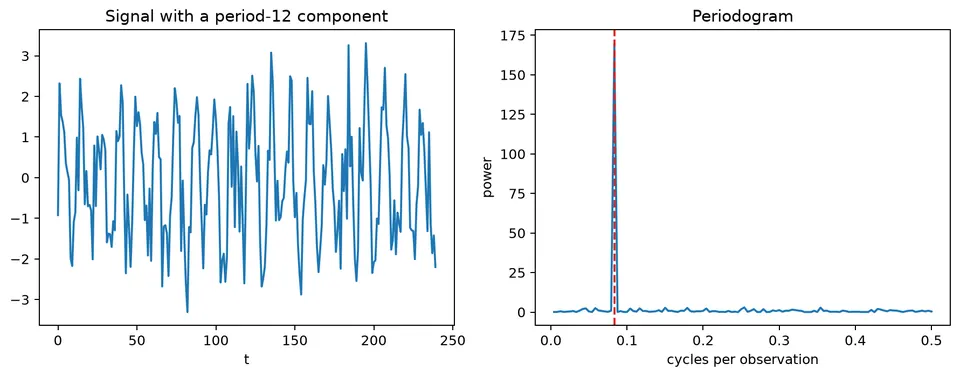
The figure connects the repeated pattern in the time domain to a concentrated peak in the frequency domain. The horizontal location of the peak gives the cycle frequency, while its inverse gives the period in observations.

Relating lags, frequencies, and periods

Time-domain methods describe dependence through lags. Frequency-domain methods describe how variation is distributed across cycles of different frequencies. These are complementary views of the same second-order structure for a stationary process.

A sinusoidal component can be written as

$$ x_t=A\cos(2\pi ft+\phi), $$

with period

$$ P=\frac{1}{f}. $$

A frequency of $1/12$ cycles per month therefore corresponds to a 12-month cycle.

Fourier Transform and Periodogram

For observations $x_0,\ldots,x_{N-1}$, the discrete Fourier transform is

$$ X_k=\sum_{t=0}^{N-1}x_te^{-i2\pi kt/N}. $$

A periodogram summarizes the squared magnitude of these Fourier components across frequency. When the autocovariances are absolutely summable, their Fourier transform gives a spectral density, and the inverse transform recovers the autocovariances. The ACF and spectrum then encode the same second-order information in different coordinates. More general weakly stationary processes have a spectral measure, which need not have an ordinary density.

One common periodogram scaling is proportional to

$$ I(f_k)=\frac{1}{N}|X_k|^2. $$

A two-sided spectrum represents both positive and negative frequencies. For real data these are paired, so a one-sided convention commonly doubles interior positive-frequency contributions while treating zero and Nyquist separately. Density scaling also accounts for sampling units. Check those conventions before comparing peak heights or integrating a spectrum to recover variance; matching peak locations alone does not establish matching normalization.

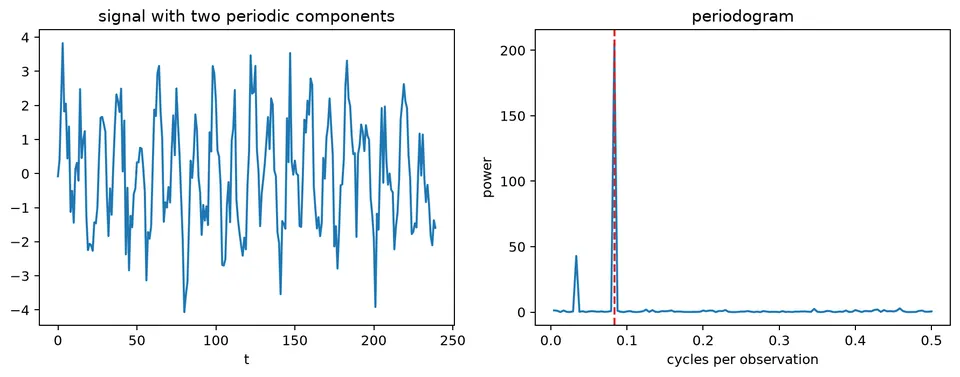
The periodogram figure shows how dominant cycle lengths appear as peaks. Because a raw periodogram is noisy, interpretation should focus on stable structure rather than treating every local maximum as a distinct physical cycle.

Nyquist Frequency and Aliasing

With one observation per sampling interval, the highest uniquely distinguishable frequency is the Nyquist frequency,

$$ f_N=\frac{1}{2} $$

cycle per interval. A higher-frequency signal can produce exactly the same sampled values as a lower-frequency signal, a phenomenon called aliasing.

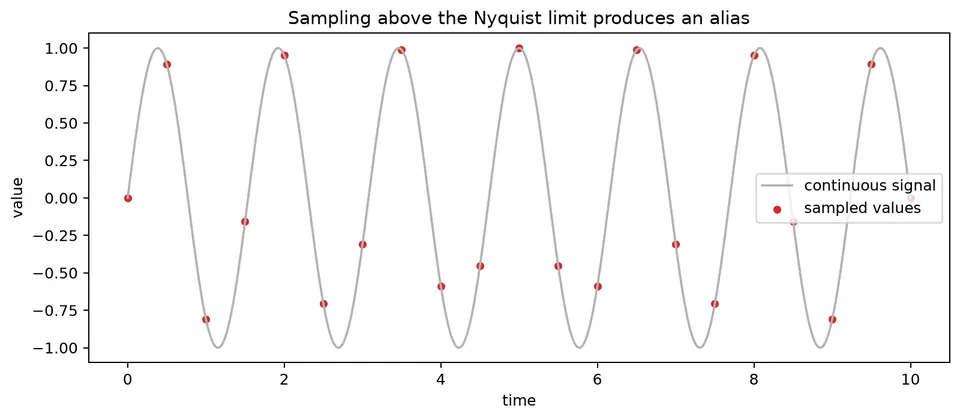
The figure demonstrates why the sampling rate must be known before assigning a physical interpretation to a spectral peak. Once a frequency has aliased into the observed band, the sampled data alone cannot recover the original higher frequency.

Spectral Leakage

The DFT represents the finite record through frequencies compatible with that record's length. A sinusoid between those grid frequencies cannot be represented by a single bin. Equivalently, truncating the sinusoid at the observation boundaries spreads its contribution across nearby frequencies. This spectral leakage can create apparent neighboring peaks even when the underlying signal contains only one oscillation.

A taper reduces the influence of the record's abrupt endpoints. It suppresses distant side lobes but broadens the central response, making closely spaced components harder to separate. Choose a window according to that tradeoff and report it when comparing spectra. A cleaner-looking plot is not automatically a more precise estimate of every frequency.

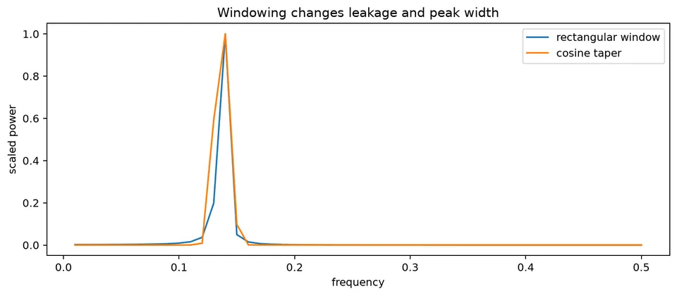
The figure shows the same underlying frequency under different window treatments. The narrower peak from a rectangular window can have stronger side lobes, while a taper suppresses those side lobes but spreads energy across a wider main peak.

A trend varies slowly and places substantial power near zero frequency. If the question concerns oscillations around that trend, model and remove the trend before examining the remainder. First differencing instead applies a known frequency-dependent filter: it suppresses low frequencies and changes the relative weighting elsewhere. The transformed spectrum therefore answers a changed question, not merely a tidier version of the original one.

For two stationary series, cross-spectral methods examine shared variation by frequency. Coherence is a frequency-specific measure of linear association, but high coherence does not establish direction or causality.

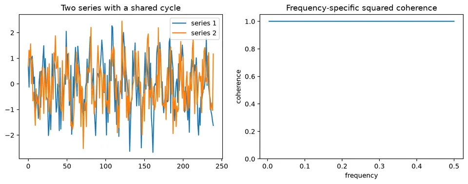
The frequency-relationship figure illustrates how two series can share a strong cycle even when their time-domain relationship is difficult to see directly.

A practical workflow is to establish the sampling interval, inspect trend and stationarity, compute a periodogram or smoothed spectrum, translate peaks into periods, and interpret them with aliasing, leakage, and multiple-search concerns in mind.

Sampling units, spectral resolution, and shared oscillations

Frequency analysis answers a different question from lag-based analysis:

At which cycle lengths is the series variable, and are those cycle lengths shared by another series?

The answer depends on the sampling rate, record length, trend treatment, windowing, and the stationarity assumptions behind the spectrum.

From period to frequency

If a pattern repeats every $P$ sampling intervals, its frequency is

$$ f=\frac{1}{P}. $$

For a 12-month cycle,

$$ f=\frac{1}{12}=0.08333 \quad\text{cycles per month}. $$

With observations every 15 minutes, a frequency of $1/12$ cycles per observation has a period of 12 observation intervals, or 3 hours. Expressed in physical units it is $1/3$ cycles per hour. Write down the sampling interval before comparing spectra from different datasets; the same numerical bin frequency can refer to entirely different physical cycle lengths.

The Nyquist frequency is half the sampling rate. With one observation per unit interval it is $0.5$ cycles per observation. A signal at $0.65$ cycles per observation is therefore observed as an alias at $|0.65-1|=0.35$ cycles per observation.

DFT and frequency resolution

For $N$ observations, the nonnegative Fourier frequencies are

$$ f_k=\frac{k}{N}, \qquad k=0,\ldots,\left\lfloor\frac{N}{2}\right\rfloor. $$

The Fourier-bin spacing is $1/N$ for a unit sampling interval. This spacing is a property of the grid; the ability to distinguish nearby physical frequencies also depends on the observation window and signal strength. With $N=240$,

$$ \Delta f=\frac{1}{240}=0.004167. $$

A period-12 component has $f=1/12$ and lies at

$$ k=Nf=240\left(\frac{1}{12}\right)=20. $$

A longer observed record makes the Fourier grid finer and can supply more complete cycles. Zero-padding the same record only interpolates its Fourier transform on a denser grid; it does not create additional observed cycles or the information of a longer record. Window broadening and noise also affect practical separation of nearby components, so bin spacing is not a complete measure of spectral resolution.

Periodogram scaling

Let $\tilde x_t=x_t-\bar x$. Its DFT is

$$ X_k=\sum_{t=0}^{N-1}\tilde x_te^{-2\pi i kt/N}. $$

A common periodogram form is

$$ I(f_k)=\frac{1}{N}|X_k|^2. $$

The constant factor varies by convention, so check the normalization before comparing absolute spectral values across software or sampling rates.

An individual raw periodogram ordinate is a noisy estimate, even with a long record. Smoothing neighboring frequencies or averaging segments reduces that variability while sacrificing some frequency resolution. A prominent peak can also come from a transient, leaked trend, or searching many frequencies. Examine whether the feature persists under reasonable estimation choices and whether its implied period is plausible in the original series.

Trend and low-frequency power

A deterministic trend changes slowly and therefore contributes strong low-frequency power. If the scientific question concerns cycles around a trend, write

$$ x_t=m_t+r_t $$

and analyze the remainder $r_t$ after estimating an appropriate trend $m_t$.

Differencing is another transformation:

$$ \nabla x_t=x_t-x_{t-1}. $$

It suppresses low frequencies but also changes the spectral shape by weighting frequencies differently. Choose the transformation because it matches the model or question, not simply because it produces a cleaner plot.

Spectral leakage and windows

A finite sample is the product of an underlying process and an observation window. A rectangular window has abrupt boundaries, so a sinusoid that does not complete an integer number of cycles spills power into neighboring Fourier bins.

A taper such as a Hann window reduces side lobes but broadens the central peak. Window choice is therefore a resolution-versus-leakage tradeoff. Report the window and detrending settings whenever spectra are compared.

Cross-spectrum and coherence

For two series $x_t$ and $y_t$, a cross-periodogram is based on

$$ I_{xy}(f)=X(f)\overline{Y(f)}. $$

Estimate coherence from smoothed or segment-averaged spectral quantities. Taking the ratio of raw single-record periodograms would give 1 wherever both DFTs are nonzero, so it would not measure the intended relationship. With appropriate spectral estimates, squared coherence has the form

$$ C_{xy}^2(f)=\frac{|S_{xy}(f)|^2}{S_{xx}(f)S_{yy}(f)}. $$

High estimated coherence means a strong linear relationship concentrated at that frequency under the spectral estimation procedure. A common annual driver can produce it in both series without a causal link between them. The squared magnitude also discards cross-spectral phase information, so it does not by itself establish which series leads. Report the smoothing or segment averaging used, and interpret any timing claim through an explicit phase convention and domain mechanism.

A numerical periodogram example

Let

$$ x_t=1.8\sin\left(\frac{2\pi t}{12}\right) +0.8\sin\left(\frac{2\pi t}{30}\right) +\varepsilon_t. $$

The first component has period 12 and the second period 30. With moderate noise, the periodogram should show peaks near

$$ \frac{1}{12}\approx0.0833 \quad\text{and}\quad \frac{1}{30}\approx0.0333. $$

The period-12 component has larger amplitude and therefore contributes more ideal sinusoidal power than the period-30 component. Noise and finite-record effects can obscure that ordering in an observed periodogram. Check the peak locations against $1/12$ and $1/30$, translate them into observation periods, and compare neighboring segments or reasonable windows to distinguish a persistent pattern from one isolated spectral feature.

Practical interpretation checklist

Before treating a spectral peak as substantive evidence:

1. verify the sampling interval and Nyquist frequency;
2. inspect the raw series and any trend or changing variance;
3. record detrending, differencing, and window settings;
4. convert the peak frequency into a period;
5. check whether the peak is near a boundary, alias, or harmonic;
6. compare adjacent time windows if stationarity is doubtful;
7. compare with an appropriate noise or domain baseline;
8. account for the number of frequencies examined;
9. avoid causal claims based on coherence alone.

The related state-space material is covered in the state-space chapter, and the state-space/frequency notebook provides an additional worked environment.

A notebook focused on the periodogram, leakage, and aliasing is frequency_domain_analysis.ipynb.

Formula reference