Binomial Distribution

A binomial random variable counts successes in a fixed number of independent trials. Each trial has two possible labels, success and failure, and the same success probability $p$. “Success” names the event being counted; it need not be desirable. Counting defective products can use exactly the same mathematics as counting products that pass inspection.

Write $X\sim\mathrm{Binomial}(n,p)$, where $n$ is a nonnegative integer and $0\le p\le1$. The possible counts are $0,1,\ldots,n$. The fixed endpoint distinguishes this model from waiting until a success occurs, where the number of trials is random.

Why the probability mass function has a binomial coefficient

One particular sequence containing $k$ successes and $n-k$ failures has probability $p^k(1-p)^{n-k}$ by independence. There are $\binom nk$ ways to choose the positions of those successes. The sequences are mutually exclusive, so their probabilities add:

$$ P(X=k)=\binom{n}{k}p^k(1-p)^{n-k},\qquad k=0,1,\ldots,n. $$

Here $\binom nk=n!/[k!(n-k)!]$. Multiplying by this coefficient is essential: “exactly $k$ successes” includes every arrangement, not just a sequence with all successes first. The probability is zero outside the support.

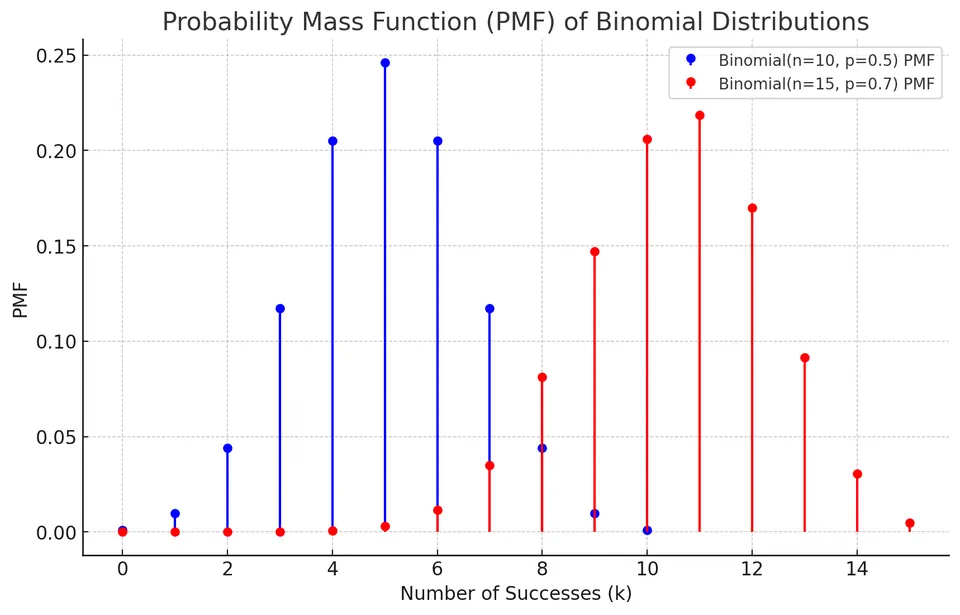
Each bar is a point probability. Its height is not an interval density, and the masses over all $n+1$ possible counts sum to 1.

Cumulative probabilities and the wording of an event

For an integer $k$ between 0 and $n$,

$$ F(k)=P(X\le k)=\sum_{i=0}^{k}\binom ni p^i(1-p)^{n-i}. $$

For a real threshold $x$, sum through $\lfloor x\rfloor$, with $F(x)=0$ below 0 and $F(x)=1$ at or above $n$. The CDF is a step function because probability accumulates only at integer counts.

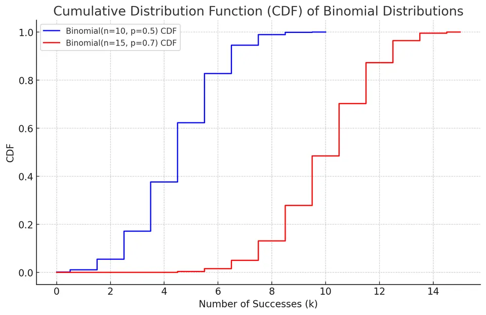
Translate the inequality before calculating. “At least 8” means $1-F(7)$; “more than 8” means $1-F(8)$; “fewer than 5” means $F(4)$. These events differ because an integer endpoint can have positive probability.

Mean, variance, and moments

Let $I_j$ be 1 when trial $j$ succeeds and 0 otherwise. Then $X=I_1+\cdots+I_n$. Each indicator has mean $p$ and variance $p(1-p)$, so

$$ E[X]=np,\qquad \mathrm{Var}(X)=np(1-p). $$

Expectation adds without requiring independence, but the variance formula uses independence to remove cross-trial covariances. A batch with correlated outcomes can have the same average success probability and a different count variance.

For one indicator, $E(e^{tI_j})=1-p+pe^t$. Independence makes the MGF of the sum the product of these factors:

$$ M_X(t)=E[e^{tX}]=(pe^t+1-p)^n,\qquad t\in\mathbb R. $$

More generally, the moment of order $m$ is $E[X^m]=M_X^{(m)}(0)$. The first two are

$$ E[X]=np,\qquad E[X^2]=np(1-p)+n^2p^2. $$

The second raw moment is not the variance: subtracting $(E[X])^2$ recovers the variance above.

Example: company email security

Suppose the probability that an audited employee follows the security protocol is $p=0.9$, and the audit examines $n=10$ employees. Model their outcomes as independent with this common probability. If the audit samples without replacement from a small company with a fixed number of compliant employees, the exact count model is hypergeometric; the binomial can be an approximation when the sampling fraction is small.

Exactly 7 compliant employees

There are $\binom{10}{7}=120$ ways to place seven compliant outcomes among ten employees:

$$ P(X=7)=\binom{10}{7}(0.9)^7(0.1)^{10-7}\approx0.0574. $$

At least 8 compliant employees

Add the mutually exclusive counts 8, 9, and 10, or subtract the probability of at most 7 from 1:

$$ P(X\ge8)=\sum_{k=8}^{10}\binom{10}{k}(0.9)^k(0.1)^{10-k}\approx0.9298. $$

Fewer than 5 compliant employees

“Fewer than 5” excludes the count 5:

$$ P(X<5)=\sum_{k=0}^{4}\binom{10}{k}(0.9)^k(0.1)^{10-k} \approx0.0001469. $$

This is about 0.0147%, or 0.0001 when the probability is rounded to four decimal places. Keeping extra digits makes the scale of this small tail probability clearer.

When the model is appropriate

Binomial counts arise in quality-control samples, fixed-size audits, survey responses, and repeated risk events when the independent, common-probability trial assumptions are defensible. A fixed number of observations alone is insufficient. Changing success probabilities or shared batch conditions change the distribution, even if the overall observed success fraction looks plausible.

Practice: Exercises with worked solutions