Hypothesis Testing

A hypothesis test compares an observed statistic with its distribution under a specified null model. A difference matters statistically when it is large relative to the variation that model predicts, rather than simply large in raw units. Applications include comparing treatments, checking production processes, and studying customer behavior. In each case, the sampling design and assumptions determine which null distribution is appropriate and how far the conclusion can be generalized.

A hypothesis is a statement about a population or statistical model that can be evaluated using data.

Inputs and Outputs of Hypothesis Testing

Inputs:

1. The null hypothesis ($H_0$) represents the default claim being tested, often stating that there is no effect or no difference.
2. The alternative hypothesis ($H_1$ or $H_a$) represents the competing claim, such as the presence of an effect or difference.
3. The significance level ($\alpha$) is a threshold chosen before examining results. A valid level-$\alpha$ test has rejection probability at most $\alpha$ under every model in the null hypothesis. Discrete procedures can have a smaller actual error rate because not every desired tail probability is attainable.
4. Sample data provide the observations used to calculate the test statistic and p-value.

Output:

The p-value is the probability, assuming the null hypothesis is true, of obtaining a test statistic at least as extreme as the one observed. A small p-value, typically $p \leq \alpha$, provides evidence against the null hypothesis.

Overview of Hypothesis Testing Steps

Hypothesis testing follows a structured process:

1. Formulate the hypotheses by defining the null and alternative hypotheses based on the research question.
2. Choose a significance level ($\alpha$), often 0.05, before examining the results.
3. Collect data using a design appropriate for the research question.
4. Calculate the test statistic using a statistical test suited to the data and assumptions.
5. Determine the p-value, which measures how unusual the observed test statistic would be if $H_0$ were true.
6. Make a decision: reject $H_0$ if the p-value is less than or equal to $\alpha$; otherwise, fail to reject $H_0$.
7. Interpret the result in the context of the research question. Failing to reject $H_0$ does not prove that it is true; it means the data do not provide sufficient evidence against it.

Example: Marble Bags

Imagine two bags: Bag A contains 5 white and 5 black marbles, while Bag B contains only black marbles.

The marble colors identify the two possible models. Draws are made with replacement so the black probability remains the same at each draw.

Suppose you want to test whether the bag is Bag B:

• The null hypothesis ($H_0$) states that the bag is Bag A.
• The alternative hypothesis ($H_a$) states that the bag is Bag B.

If we draw n marbles independently with replacement and they are all black, we can evaluate how likely this result would be under $H_0$.

For Bag A, the probability of drawing a black marble is 0.5. Therefore, the probability of drawing n black marbles in a row is:

$$ (0.5)^n $$

• For $n=2$, p-value $=(0.5)^2=0.25$
• For $n=3$, p-value $=(0.5)^3=0.125$
• For $n=5$, p-value $=(0.5)^5=0.03125$

A smaller p-value provides stronger evidence against $H_0$. As n increases, observing only black marbles becomes increasingly difficult to explain if the bag is Bag A.

Take the number of black draws as the statistic and large counts as evidence toward Bag B. For a sample of fixed size $n$, all $n$ draws being black is the largest possible count, so the relevant upper tail consists of that outcome alone and equals $(1/2)^n$. The p-value is not the posterior probability of Bag A: that would also require prior probabilities for the bags. The calculation assumes $n$ was fixed in advance. Repeatedly testing and stopping when a small p-value appears changes the procedure and can inflate its false-positive rate.

Null and Alternative Hypotheses for a Mean

When testing a population mean, three common forms of hypotheses are used.

Types of Tests

I. Left-Tailed Test

• The null hypothesis ($H_0$) states that the population mean $\mu$ equals a specified value $\mu_0$:

$$ \mu=\mu_0 $$

• The alternative hypothesis ($H_a$) states that:

$$ \mu<\mu_0 $$

II. Right-Tailed Test

• The null hypothesis ($H_0$) states that:

$$ \mu=\mu_0 $$

• The alternative hypothesis ($H_a$) states that:

$$ \mu>\mu_0 $$

III. Two-Tailed Test

• The null hypothesis ($H_0$) states that:

$$ \mu=\mu_0 $$

• The alternative hypothesis ($H_a$) states that:

$$ \mu\neq\mu_0 $$

For one-sided alternatives, the null is often written as $\mu\ge\mu_0$ (left-tailed) or $\mu\le\mu_0$ (right-tailed). The test statistic and p-value are computed at the boundary value $\mu=\mu_0$, which is the least favorable case for rejecting $H_0$, so writing $H_0:\mu=\mu_0$ gives the same test.

The alternative hypothesis determines whether the test examines values below, above, or on either side of $\mu_0$.

Important Note: Left-tailed and right-tailed tests are appropriate when the research question specifies a meaningful direction in advance. A two-tailed test is used when departures in either direction are relevant.

Examples

I. Testing the Effectiveness of a New Diet (Two-Tailed Test)

• The null hypothesis ($H_0$) is that the average daily energy expenditure $\mu$ equals the standard-diet average $\mu_0$.
• The alternative hypothesis ($H_a$) is that the average daily energy expenditure differs from the standard-diet average:

$$ \mu\neq\mu_0 $$

II. Evaluating Customer Service Efficiency (Left-Tailed Test)

• The null hypothesis ($H_0$) states that the average resolution time is 10 minutes:

$$ \mu=10 $$

• The alternative hypothesis ($H_a$) states that the average resolution time is less than 10 minutes:

$$ \mu<10 $$

III. Assessing the Impact of a New Teaching Method (Right-Tailed Test)

• The null hypothesis ($H_0$) states that the average test score equals the district average of 75%:

$$ \mu=75 $$

• The alternative hypothesis ($H_a$) states that the average test score exceeds 75%:

$$ \mu>75 $$

The P-value

After collecting the data and calculating the test statistic, the researcher computes the p-value.

The p-value is the probability, assuming the null hypothesis is true, of obtaining a test statistic at least as extreme as the one observed.

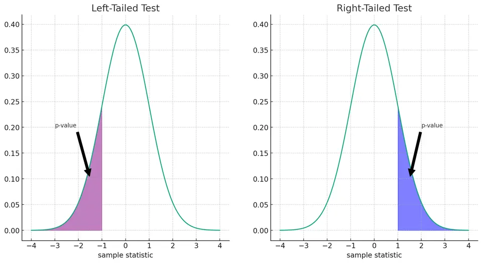
• In a left-tailed test, the p-value is the area in the left tail beyond the observed test statistic.
• In a right-tailed test, the p-value is the area in the right tail beyond the observed test statistic.

For a two-tailed test, extreme values in both directions are considered. For a symmetric reference distribution such as the standard normal or $t$, the two-tailed p-value is $2P(T\ge|t_{\mathrm{obs}}|)$.

Here, "at least as extreme" means values at least as inconsistent with $H_0$ as the observed result, according to the alternative hypothesis.

Choosing the Right Statistical Test

Selecting an appropriate statistical test depends on the type of data, research question, study design, and assumptions.

Factors to Consider

1. The type of data influences which statistical methods are appropriate. Numerical, categorical, and ordinal variables are analyzed differently.
2. The number of variables or groups affects the choice of test.
3. The distribution and assumptions of the statistical model must be considered. Some parametric methods rely on assumptions such as approximate normality, while non-parametric methods generally make fewer distributional assumptions.
4. The study design, such as whether groups are independent or measurements are paired, also determines which test is appropriate.

Examples of Statistical Tests

• An independent-samples t-test compares two means, with Welch's version allowing unequal variances. The Mann-Whitney U test addresses equality of distributions or a rank-based ordering question under its assumptions. It is not automatically a test of the same mean difference, and a median-shift interpretation requires additional shape assumptions. Choose a method by the target quantity, not solely by whether a normality check rejects.
• To compare means across more than two groups, Analysis of Variance (ANOVA) is commonly used.
• For categorical count data, a chi-square test can be used to examine distributions or associations.
• Left-tailed and right-tailed tests correspond to directional alternative hypotheses.
• Two-tailed tests are used when departures in either direction are relevant.
• Parametric tests rely on a specified statistical model, while non-parametric tests generally require fewer distributional assumptions.

The following table summarizes some common statistical tests and their applications:

Example: Hypothesis Test for the Mean

An agronomist asks whether mean yield under a new fertilizer exceeds a fixed reference of 2 tons per hectare. The fertilizer is applied to randomly selected plots from the target population. This one-sample design compares the treated-condition mean with the reference; establishing the fertilizer's causal effect relative to no fertilizer would require a suitable control comparison or additional assumptions.

The yield of 25 plots is measured, giving:

• Sample mean: $\bar{x}=2.1$ tons per hectare
• Sample standard deviation: $s=0.3$ tons per hectare
• Sample size: $n=25$
• Significance level: $\alpha=0.05$

Hypothesis Setup:

• Null Hypothesis ($H_0$):

$$ \mu=2 $$

• Alternative Hypothesis ($H_a$):

$$ \mu>2 $$

Test Statistic:

Assume the plot yields are independent and their population distribution is approximately normal, without influential outliers. Under these conditions, estimating the unknown standard deviation with $s$ leads to a one-sample t statistic. For an exactly normal population its null distribution is exactly $t_{n-1}$; for other populations the approximation depends on the data and sample size:

$$ t=\frac{\bar{x}-\mu_0}{s/\sqrt{n}} $$

where:

• $\bar{x}$ is the sample mean,
• $\mu_0$ is the hypothesized population mean,
• $s$ is the sample standard deviation,
• $n$ is the sample size.

Plugging in the values:

$$ t=\frac{2.1-2}{0.3/\sqrt{25}} $$

$$ t=\frac{0.1}{0.06} $$

$$ t\approx1.667 $$

The test has:

$$ df=n-1=24 $$

For a right-tailed test with $\alpha=0.05$ and 24 degrees of freedom, the critical value is approximately:

$$ t^*\approx1.711 $$

Since:

$$ 1.667<1.711 $$

we fail to reject the null hypothesis.

The corresponding one-sided p-value is $P(T_{24}\ge1.667)\approx0.054$, which is just above $0.05$, so the conclusion is the same.

There is insufficient evidence at the $\alpha=0.05$ level to conclude that mean yield under the fertilizer exceeds 2 tons per hectare. The estimated excess is still $0.1$ ton per hectare, and the result is near the chosen threshold. Reporting the estimate, its uncertainty, and the p-value conveys more than labeling it nonsignificant. The test does not establish that the excess is zero or that the fertilizer has no useful effect.

Effect Size and Practical Significance

A statistically significant result does not necessarily imply a practically meaningful one. Effect size describes the magnitude of a difference or relationship and helps assess whether an observed effect is large enough to matter in practice.

Cohen's d

Cohen's $d$ is a commonly used effect-size measure for comparing two means. It expresses the difference between the means in units of the pooled standard deviation:

$$ d = \frac{\bar{x}_1 - \bar{x}_2}{s_p} $$

where $s_p$ is the pooled standard deviation:

$$ s_p = \sqrt{\frac{(n_1 - 1) s_1^2 + (n_2 - 1) s_2^2}{n_1 + n_2 - 2}} $$

Common benchmarks for interpreting $|d|$ are:

These values are rough conventions rather than universal thresholds.

Because the p-value depends on both the size of the effect and the amount of data, a large sample can produce a statistically significant result even when the effect is small. Reporting an effect size alongside the p-value gives a more complete picture of the findings.

The SciPy Mann-Whitney documentation distinguishes the distributional null from more restrictive location interpretations and describes the independent-sample requirement.