Poisson Distribution

A Poisson random variable counts events in a specified interval of time, distance, area, or other exposure. Write $X\sim\mathrm{Poisson}(\lambda)$, where $\lambda$ is the expected count in that interval. Its support is $\{0,1,2,\ldots\}$: there is no fixed number of trials that caps the count.

A constant-rate Poisson process supplies one mechanism for this distribution. Counts in disjoint intervals are independent, and their mean is proportional to exposure. If the process rate is $r$ events per hour and an interval lasts $T$ hours, the count parameter is $\lambda=rT$. The rate and the expected count coincide numerically only when the exposure is one unit.

Probability mass function

For $\lambda>0$,

$$ P(X=k)=\frac{e^{-\lambda}\lambda^k}{k!},\qquad k=0,1,2,\ldots. $$

The masses sum to 1 because $\sum_{k=0}^\infty\lambda^k/k!=e^\lambda$, canceling the factor $e^{-\lambda}$. At $\lambda=0$, the limiting distribution assigns probability 1 to zero events.

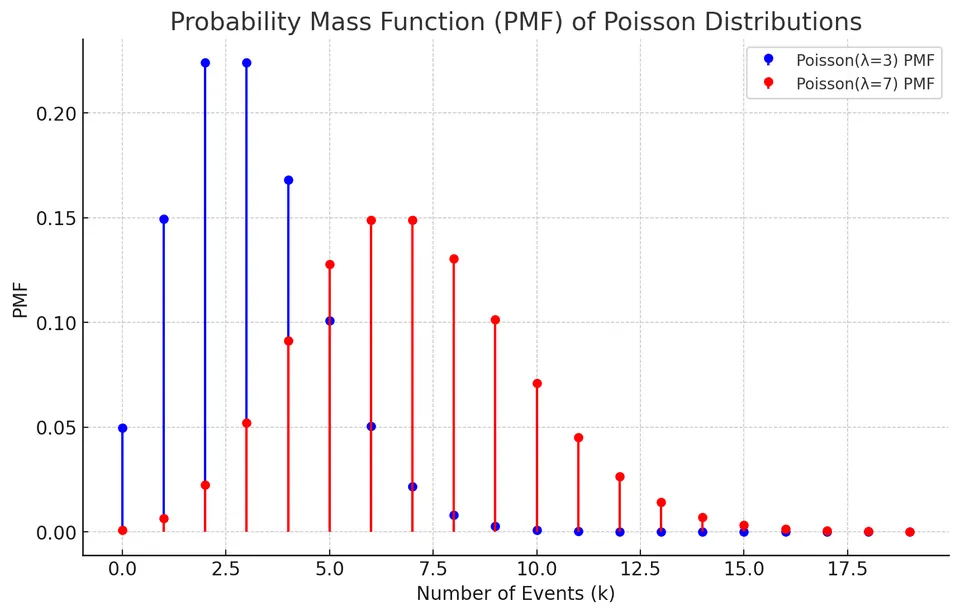
Poisson probability masses for nonnegative event counts

As exposure grows at the same rate, the expected count grows. A mean of five events in an hour does not mean that five events occur in every hour; the PMF describes the variability around that mean.

Cumulative probabilities

For a nonnegative integer $k$,

$$ F(k)=P(X\le k)=\sum_{i=0}^{k}\frac{e^{-\lambda}\lambda^i}{i!}. $$

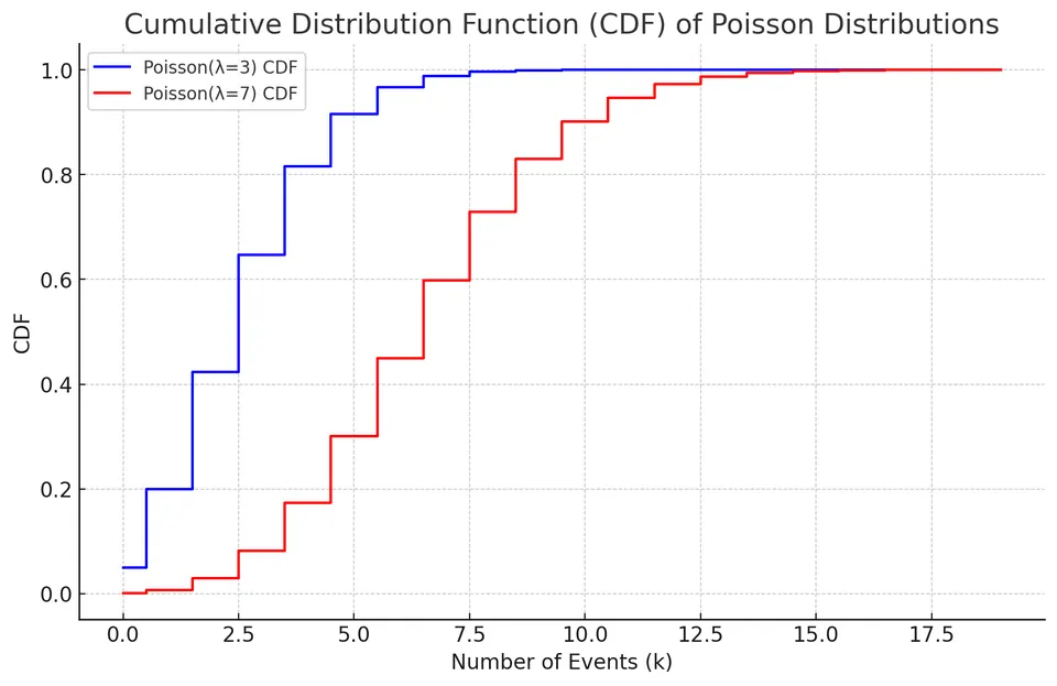
For real $x\ge0$, sum through $\lfloor x\rfloor$; for $x<0$, the CDF is zero. “More than $k$” uses the complement $1-F(k)$, whereas “at least $k$” uses $1-F(k-1)$.

Poisson CDF accumulating probability at integer counts

Mean, variance, and moments

The Poisson model imposes the same value for its mean and variance:

$$ E[X]=\mathrm{Var}(X)=\lambda. $$

This is a modeling restriction, not an identity for all count data. Changing rates across observation periods or clustered arrivals can produce much more variability than this one-parameter model permits.

The MGF follows by collecting the exponential series:

$$ M_X(t)=E[e^{tX}]=e^{\lambda(e^t-1)},\qquad t\in\mathbb R. $$

Differentiating once gives $M'_X(t)=\lambda e^tM_X(t)$. Differentiating again and setting $t=0$ gives the first two raw moments:

$$ E[X]=\lambda,\qquad E[X^2]=\lambda^2+\lambda. $$

More generally, $E[X^m]=M_X^{(m)}(0)$. Subtracting $\lambda^2$ from the second moment recovers the variance $\lambda$.

Suppose accident-related visits average 5 per hour and a constant-rate Poisson model is appropriate over the periods studied. For a one-hour interval, $\lambda=5$. This is a model for visits, which need not equal the number of distinct accidents.

Exactly 3 visits in an hour

$$ P(X=3)=\frac{e^{-5}5^3}{3!}\approx0.1404. $$

More than 7 visits in an hour

The complement includes counts 0 through 7:

$$ P(X>7)=1-\sum_{k=0}^{7}\frac{e^{-5}5^k}{k!}\approx0.1334. $$

At most 2 visits in an hour

$$ P(X\le2)=\sum_{k=0}^{2}\frac{e^{-5}5^k}{k!}\approx0.1247. $$

For a half-hour interval the expected count would be $5(0.5)=2.5$, not 5. Adjusting exposure is part of specifying the distribution before applying its formulas.

Poisson approximation to a binomial count

For many independent trials with small success probability, keep $\lambda=np$ fixed or moderate while increasing $n$ and decreasing $p$. For each fixed count, the binomial probability approaches the corresponding Poisson probability:

$$ \mathrm{Binomial}(n,p)\approx\mathrm{Poisson}(np). $$

The approximation replaces a large collection of rare trial events with an event-count model. It is not appropriate merely because a binomial mean is known: a large success probability or a count near the finite upper limit can make the Poisson approximation poor.

Practice: Exercises with worked solutions