Randomness and Trend Tests

A noisy-looking plot can still contain structure. Consecutive values may cluster on one side of the mean, changes may alternate unusually often, or large residuals may arrive together. A diagnostic test turns one such observation into a defined statistic and compares it with a reference distribution under a specific null hypothesis.

There is no universal null called “randomness” that every test examines. The Ljung-Box statistic targets selected linear autocorrelations. Turning-point and runs statistics target ordering. A rank statistic targets monotone association with time. A squared-residual diagnostic targets dependence in magnitude.

Choose the diagnostic after stating what a model is supposed to explain. For a conditional-mean model, ordinary residual correlation is relevant. For a volatility model, dependence in squared standardized residuals matters too. A rejection identifies a kind of mismatch, while failure to reject can reflect either compatibility with the null or a sample too weak to detect the alternative. Interpret the statistic alongside its assumptions and the residual plot.

Worked calculation: counting turning points

For the short sequence

$$ 1,\ 3,\ 2,\ 4,\ 3, $$

the interior observations at positions 2, 3, and 4 are all turning points: position 2 (value 3) is a peak, position 3 (value 2) is a trough, and position 4 (value 4) is a peak. Thus the count is 3. A turning-point test compares the observed count with the distribution expected under a continuous IID null; it is not a general test of every possible dependence pattern.

For a fitted model, the more important question is whether residuals still contain predictable structure. A residual ACF, a Ljung-Box test, and a plot of squared residuals address different kinds of remaining dependence and should be interpreted together.

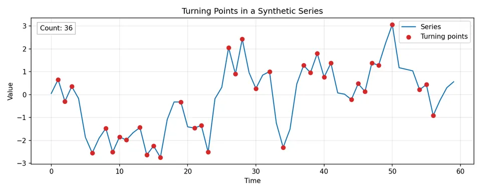
The figure marks local peaks and troughs directly. A sequence with unusually few turning points tends to move persistently in one direction, while unusually many turning points indicate excessive alternation.

What each diagnostic tests

When a series looks noisy, diagnostics can still test whether particular forms of structure remain. Start by stating the null hypothesis, the lags or ordering features examined, and the sample to which the test is applied. A result for raw observations answers a different question from a result for fitted innovation residuals. No single procedure proves randomness across every possible form of dependence.

Ljung-Box Q test: joint autocorrelation

The Ljung-Box test pools information from the first $m$ sample autocorrelations. Squaring makes positive and negative correlations contribute in the same direction; otherwise they could cancel. The factors involving $n$ and $n-k$ adjust the basic sum for finite-sample behavior. The resulting statistic checks whether the tested correlations are jointly compatible with zero:

$$ Q=n(n+2)\sum_{k=1}^{m}\frac{\hat r_k^2}{n-k}, $$

where $\hat r_k$ is the sample autocorrelation at lag $k$ and $m$ is the maximum lag included in the test.

Under an appropriate IID null, $Q$ is commonly compared with a $\chi^2_m$ approximation. Fitted residuals are different because estimating the model has already used some of the correlation information. For ARMA($p,q$) residuals a common adjustment uses $m-p-q$ degrees of freedom, requiring $m>p+q$. Choose the lag range and adjustment for the fitted model and sampling frequency rather than accepting a software default without interpretation.

A rejection means that at least some of the tested linear autocorrelations are inconsistent with the null. It does not identify which new model should be fitted. Failure to reject only means that this set of lag correlations has not supplied enough evidence against the null; nonlinear dependence, untested seasonal lags, and low power in a short sample can remain relevant.

McLeod-Li Test (Squared Series)

The McLeod-Li test applies a Ljung-Box-type statistic to squared observations or squared residuals:

$$ Q_{\mathrm{ML}}=n(n+2)\sum_{k=1}^{m}\frac{\hat r_{k,\mathrm{sq}}^2}{n-k}. $$

Squaring removes the sign of a residual and emphasizes its magnitude. If positive and negative errors cancel in the ordinary ACF but large squared errors cluster, a mean model can pass a linear-correlation check while leaving variance dynamics unexplained. ARCH or GARCH may then be candidates, but breaks and outliers can also produce squared-residual correlation. The test indicates a feature to investigate, not a unique variance equation.

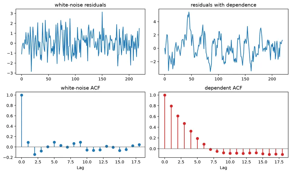
The figure places mean-dependence and variance-dependence diagnostics side by side. Residual autocorrelation points to structure left in the conditional mean, while autocorrelation in squared residuals points to time-varying conditional variance.

Turning Point Test (IID vs. Not IID)

A turning point occurs at an interior time $t$ when the series changes direction:

$$ (x_{t-1}<x_t>x_{t+1}) \quad\text{or}\quad (x_{t-1}>x_t<x_{t+1}). $$

Let $T$ be the number of turning points in a series of length $n$. For a continuous IID sequence with $n\ge4$, the reference moments are

$$ E(T)=\frac{2(n-2)}{3}, \qquad \mathrm{Var}(T)=\frac{16n-29}{90}. $$

A standardized statistic

$$ \frac{T-E(T)}{\sqrt{\mathrm{Var}(T)}} $$

can be compared with a normal approximation when the record is sufficiently long. The expected proportion $2/3$ has a simple explanation: among three independent continuous observations, the middle position is equally likely to contain the smallest, middle, or largest value; it is a turning point in two of those three cases. Ties and overlapping triples affect the reference calculation, which is why the stated variance is not a binomial variance.

The worked example and figure above show exactly what is being counted.

Sign changes in successive differences

Successive differences are

$$ d_t=x_t-x_{t-1}, \qquad t=2,\ldots,n. $$

For nonzero differences, define

$$ s_t=\mathrm{sign}(d_t)\in\{-1,+1\}. $$

A change of sign between adjacent differences occurs when

$$ s_t\ne s_{t-1}. $$

With no ties, this event is exactly a turning point of the original series. Therefore the count

$$ C=\sum_{t=3}^{n}I(s_t\ne s_{t-1}) $$

has the same continuous-IID reference moments as the turning-point count (with the displayed variance formula applying for $n\ge4$):

$$ E(C)=\frac{2(n-2)}{3}, \qquad \mathrm{Var}(C)=\frac{16n-29}{90}. $$

The signs of successive differences are not independent under an IID level series because adjacent differences share an observation. Treating them as independent fair coin flips would give the wrong reference distribution for this particular statistic. This section counts changes between difference signs. A test that instead counts positive differences is a different statistic and requires its own reference distribution.

Rank Test (Detecting Trend)

A rank-based trend test looks for monotone association between time and the observed values without requiring a normal marginal distribution.

If there are no ties, replace the observations by ranks $r_t$ and compute Spearman's rank correlation between time and rank:

$$ \rho_s=1-\frac{6\sum_{t=1}^{n}(r_t-t)^2}{n(n^2-1)}. $$

A large magnitude of Spearman correlation means that larger ranks tend to occur systematically earlier or later in the record. Ranks make the statistic less sensitive to the size of an extreme value, but they do not distinguish a smooth trend from a sudden level shift. Tied values need adjusted ranks, and serial dependence changes ordinary independent-sample significance calculations. Separate the descriptive rank association from the assumptions of the trend test used to assess it.

Because several diagnostics are often applied to the same series, isolated p-values should not be interpreted as independent discoveries. Use the tests as targeted checks and relate them to plots, model assumptions, and forecast performance.

Interpreting counts, rejections, and residual evidence

There is no single test that proves a time series is random. Different diagnostics ask different questions:

• are values linearly dependent across selected lags?
• are there too many or too few turning points?
• is there a monotone trend?
• are squared residuals dependent?
• is a unit-root or stationarity null compatible with the data?

Choose the diagnostic to match the model failure that matters.

Turning points

For

$$ 1,\ 3,\ 2,\ 4,\ 3, $$

the interior observations at positions 2, 3, and 4 are local turning points, so $T=3$. Too few turning points can indicate persistence or trend; too many can indicate alternation or negative dependence. The test does not identify the mechanism responsible for the departure.

Runs

Convert observations to signs relative to a reference level, often the median. A run is a maximal sequence of identical signs. For

$$ ++--+--, $$

there are four runs: $++$, $--$, $+$, and $--$. The count records how often the sign sequence switches, not how far values lie from the reference level. Here there are three positive and four negative signs; under a random ordering conditional on those counts, the expected number of runs is $1+2(3)(4)/7\approx4.43$. Four runs is therefore not automatically suspicious. A formal conclusion needs the relevant small-sample distribution or a justified approximation.

Ljung-Box residual test

The Ljung-Box statistic through lag $m$ is

$$ Q(m)=n(n+2)\sum_{h=1}^{m}\frac{\hat\rho(h)^2}{n-h}. $$

A p-value of 0.002 indicates that the observed aggregate correlation is unusual under the specified zero-correlation reference, including the fitted-model adjustment. It does not mean that the probability of the model being correct is 0.002, nor does it identify the problematic lag. Inspect the residual correlogram to distinguish short-lag, seasonal, and broad persistent patterns before changing the model.

Trend tests and breaks

A monotone trend test can be useful when a linear trend is not justified, but a smooth trend and a structural break can look similar in a short record. Plot the series, rolling summaries, and residuals around any suspected change before attributing a rejection to one particular mechanism.

Multiple diagnostics

If ten independent tests were each run at level $0.05$, the probability of at least one false rejection would be

$$ 1-(1-0.05)^{10}\approx0.401. $$

The calculation is an illustration under independent tests, not an exact error rate for a collection of dependent time-series diagnostics. Its practical lesson is to avoid searching through many lags, transformations, and tests until one p-value looks striking. State the failures being checked, report the related evidence together, and investigate whether the proposed model change improves residual behavior and later forecasts.

A practical diagnostic sequence

1. Inspect the raw series and timestamp structure.
2. Model or remove known trend and seasonality when appropriate.
3. Inspect the residual ACF and Ljung-Box results.
4. Inspect squared residuals for variance dependence.
5. Use turning-point or runs tests as complementary ordering checks.
6. Investigate breaks, outliers, and changes in variance.
7. Validate the resulting model with temporal forecast evaluation.

Formula reference