Exponential Distribution
The exponential distribution models the wait to the next event in a constant-rate Poisson process. Write $X\sim\mathrm{Exp}(\lambda)$ with rate $\lambda>0$. If time is measured in years, $\lambda$ has units of events per year and $X$ has units of years. Larger rates mean shorter typical waits.
The model permits any positive wait rather than a fixed lifetime. Its constant hazard means that surviving for some time does not change the distribution of the remaining wait. That is a substantive assumption for a physical lifetime: an aging or wearing component need not follow it.
From no events to the CDF and density
The event $X>x$ means that no Poisson event occurs during the first $x$ time units. The expected event count over that interval is $\lambda x$, and the zero-count probability is $e^{-\lambda x}$. Thus
$$ P(X>x)=e^{-\lambda x},\qquad x\ge0. $$
Taking the complement gives the CDF:
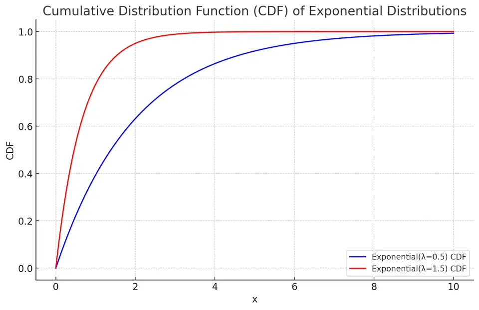
$$ F(x)=1-e^{-\lambda x},\qquad x\ge0, $$
with $F(x)=0$ for $x<0$. Differentiating the CDF on the positive half-line gives
$$ f(x)= \begin{cases} \lambda e^{-\lambda x},&x\ge0,\\ 0,&x<0. \end{cases} $$
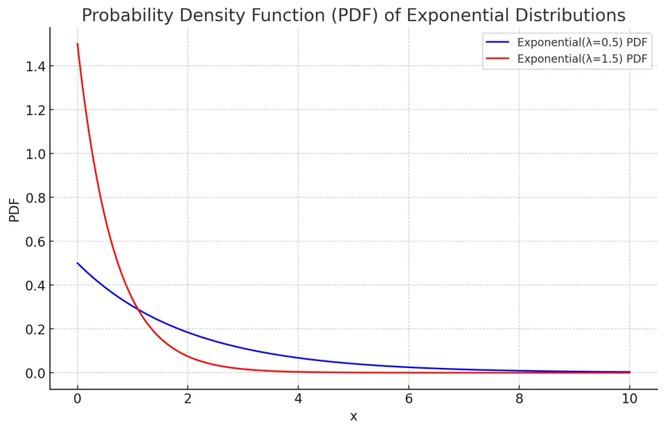
The density height is not the probability of failing at exactly that time. Interval probabilities are areas, or differences of CDF values.
Memorylessness
For nonnegative $s$ and $t$,
$$ P(X>s+t\mid X>s)=\frac{e^{-\lambda(s+t)}}{e^{-\lambda s}} =e^{-\lambda t}=P(X>t). $$
Conditioning on survival through $s$ leaves the same probability of waiting more than another $t$. This does not mean that a survivor starts its physical life over; it states that elapsed age carries no predictive information about the remaining lifetime under the exponential model.
Mean, variance, and moments
The expected wait and its variance are
$$ E[X]=\frac1\lambda,\qquad \mathrm{Var}(X)=\frac1{\lambda^2}. $$
The standard deviation equals the mean, showing that the distribution permits substantial variation even with one fixed rate. A mean lifetime is not a deadline by which every component has failed.
To derive moments, integrate the exponentially weighted density:
$$ M_X(t)=E[e^{tX}]=\int_0^\infty \lambda e^{-(\lambda-t)x}\,dx =\frac{\lambda}{\lambda-t},\qquad t<\lambda. $$
The integral converges only when $\lambda-t>0$. Differentiating gives
$$ E[X^n]=\frac{d^nM_X(t)}{dt^n}\Bigg|_{t=0} =\frac{n!}{\lambda^n},\qquad n=0,1,2,\ldots. $$
In particular,
$$ E[X]=\frac1\lambda,\qquad E[X^2]=\frac2{\lambda^2}. $$
Subtracting the squared mean from the second raw moment leaves $1/\lambda^2$, the variance above.
Example: equipment failure times
An engineer models a component's lifetime as exponential with mean 5 years. The rate is therefore $\lambda=1/5=0.2$ per year, not 5 per year.
Failure within the first year
Use the CDF because the event is a wait below a threshold:
$$ P(X<1)=1-e^{-1/5}\approx0.1813. $$
There is about an 18.13% probability of failure in the first year under this model. Replacing $<$ with $\le$ does not change the result because an exact time has zero probability.
Lasting more than 10 years
Use the survival probability directly:
$$ P(X>10)=e^{-10/5}=e^{-2}\approx0.1353. $$
About 13.53% of modeled lifetimes exceed 10 years. If a component has already survived 10 years, its remaining lifetime still has mean 5 years under the memoryless assumption; it is not forced to fail immediately because it exceeded the original mean.
Applications
Exponential waits appear in queueing, reliability, and survival models with an approximately constant event hazard. Independent equal-rate exponential stages sum to a gamma distribution. When the rate changes with age or operating conditions, that change needs its own model rather than being hidden inside a single average lifetime.
Practice: Exercises with worked solutions