Forecasting with Time Series

A forecast answers a dated question: what can be said about a specified future quantity using the information available now? Predicting next month's total sales from today's data is different from predicting tomorrow's sales, and both differ from estimating a past trend with the full record available. The forecast origin, horizon, units, and information set are part of the question.

A point forecast also needs a target. The conditional mean minimizes expected squared error; a conditional median minimizes expected absolute error; a quantile answers a tail-probability question. Those values can differ for an asymmetric forecast distribution, so one number cannot automatically serve all three purposes.

Forecasting methods specify what persists: the latest level, an estimated trend, a seasonal pattern, a dynamic response to past shocks, or a relationship with predictors. Their usefulness depends on whether that assumption holds over the required horizon. Compare methods against appropriate baselines at historical forecast origins, and assess the uncertainty distribution as well as the point errors.

Worked calculation: a forecast and its uncertainty

For a centered AR(1),

$$ X_t=0.8X_{t-1}+\varepsilon_t, \qquad \mathrm{Var}(\varepsilon_t)=1, $$

if the latest observation is $X_T=5$, then

$$ \hat X_{T+1|T}=0.8(5)=4, \qquad \hat X_{T+5|T}=0.8^5(5)=1.6384. $$

The $h$-step forecast-error variance is

$$ \mathrm{Var}(X_{T+h}-\hat X_{T+h\mid T}) =\sum_{j=0}^{h-1}0.8^{2j}. $$

At $h=2$,

$$ \mathrm{Var}(e_{T+2})=1+0.8^2=1.64, $$

so an approximate Gaussian 95% prediction interval around the two-step forecast $0.8^2(5)=3.2$ uses

$$ 3.2\pm1.96\sqrt{1.64}\approx3.2\pm2.51, $$

that is, roughly $(0.69,\,5.71)$.

The centered AR(1) forecast multiplies the latest value by another factor of 0.8 for each step, so it returns toward zero. Uncertainty moves in the other direction because each step introduces an additional unknown shock. By the second step, one future shock enters directly and one is multiplied by 0.8; their variance contributions are $1$ and $0.8^2$. This explains the variance 1.64 and the interval calculation above.

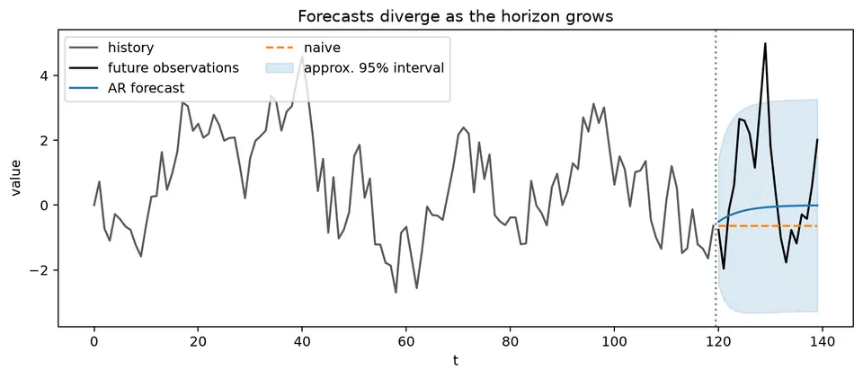
The figure shows both parts of a forecast. The central path gives the conditional mean, while the widening interval reflects uncertainty from future shocks that have not yet been observed.

The forecast target and available information

Time-series forecasting predicts future observations using information available at a specified forecast origin. A forecast is therefore not only a model output; it is a conditional statement tied to a horizon, an information set, and an uncertainty estimate.

Components of a Time Series

Forecasting methods differ in how they represent trend, seasonality, cycles, and irregular variation. Identifying these structures first helps determine which model class and baseline are appropriate.

Trend is a persistent long-run movement in level or slope.

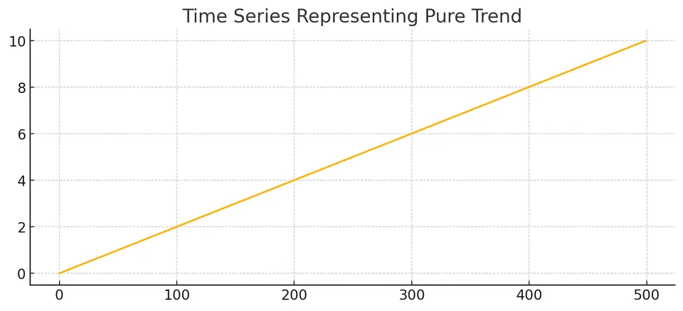
The trend figure shows a systematic change in the level. A level-only forecasting method will lag behind such movement unless a trend component or transformation is included.

Seasonality is a pattern that repeats at a fixed period such as day of week, month of year, or quarter.

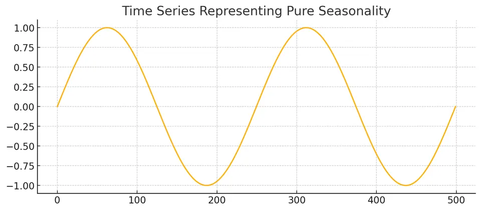
The repeated spacing of peaks and troughs suggests a seasonal model or seasonal baseline rather than an ordinary non-seasonal trend model.

Cycles are oscillations whose duration is not tied to one fixed seasonal period.

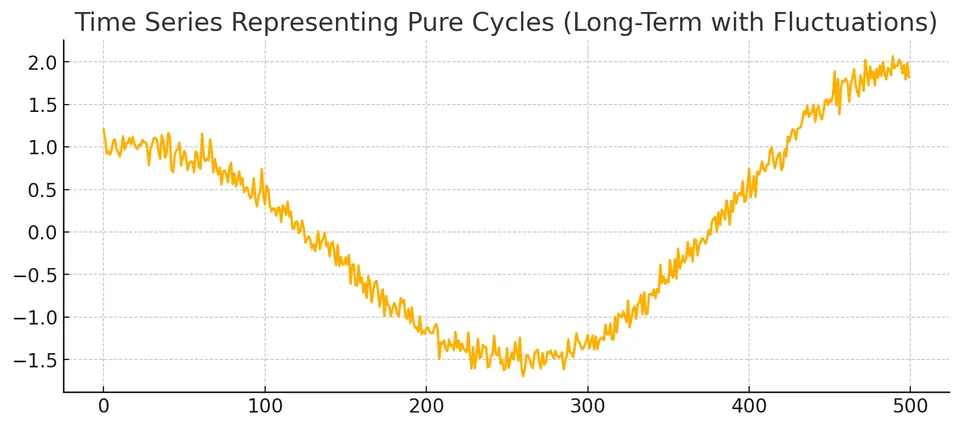
Because cycle length can vary, long-range cyclic behavior is usually harder to extrapolate reliably than fixed calendar seasonality.

The irregular component is the variation not explained by the chosen systematic structure.

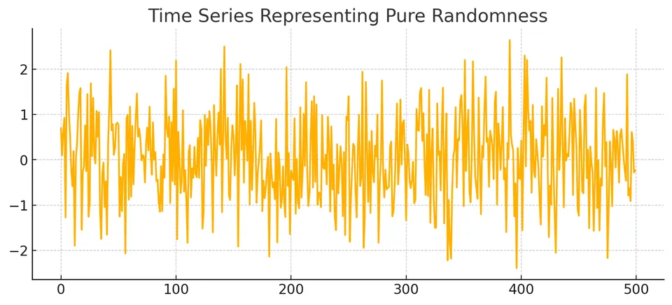
A remainder should be checked rather than assumed to be random. Residual autocorrelation, changing variance, or heavy tails indicate structure that the forecasting model has not yet captured.

Forecasting Methods

Forecasting methods encode different assumptions about persistence, level, trend, seasonality, and nonlinear dependence. Start with a simple baseline, then add complexity only when it improves predictions made at historical forecast origins or provides necessary probabilistic structure.

Naive Forecast

The naive forecast assumes that the latest observed level persists:

$$ \hat y_{t+h\mid t}=y_t. $$

For one step ahead this is simply

$$ \hat y_{t+1\mid t}=y_t. $$

It is a strong baseline for persistent non-seasonal series and is the optimal conditional-mean forecast for a zero-drift random walk.

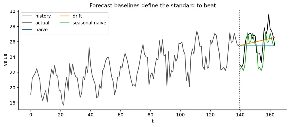
The figure compares several simple rules. Naive, seasonal-naive, mean, and drift forecasts correspond to different assumptions about what persists into the future, so the benchmark should match the basic structure of the series.

Simple Exponential Smoothing (SES)

Simple exponential smoothing (SES) maintains one estimate of the current level. A new observation revises that estimate rather than triggering an extrapolation of a permanent slope. The update below is equivalent to “previous level plus $\alpha$ times the new prediction error.” This makes the role of $\alpha$ concrete: it controls how much of the latest surprise is treated as a change in level.

$$ \ell_t=\alpha x_t+(1-\alpha)\ell_{t-1}, \qquad 0<\alpha\le1, $$

and the level-only forecast is

$$ \hat x_{t+h\mid t}=\ell_t. $$

If $\alpha$ is large, a new surprise moves the level substantially. If it is small, the level changes slowly and averages information over a longer history. Neither behavior is automatically better. A rapidly changing underlying level needs responsiveness; measurement noise can make that same responsiveness chase temporary fluctuations. Choose the parameter through fitting and temporal evaluation rather than through the visual smoothness of the curve.

Repeated substitution gives

$$ \ell_t =\alpha x_t +\alpha(1-\alpha)x_{t-1} +\alpha(1-\alpha)^2x_{t-2} +\cdots, $$

up to the contribution from the initial state. The observation weights decay geometrically.

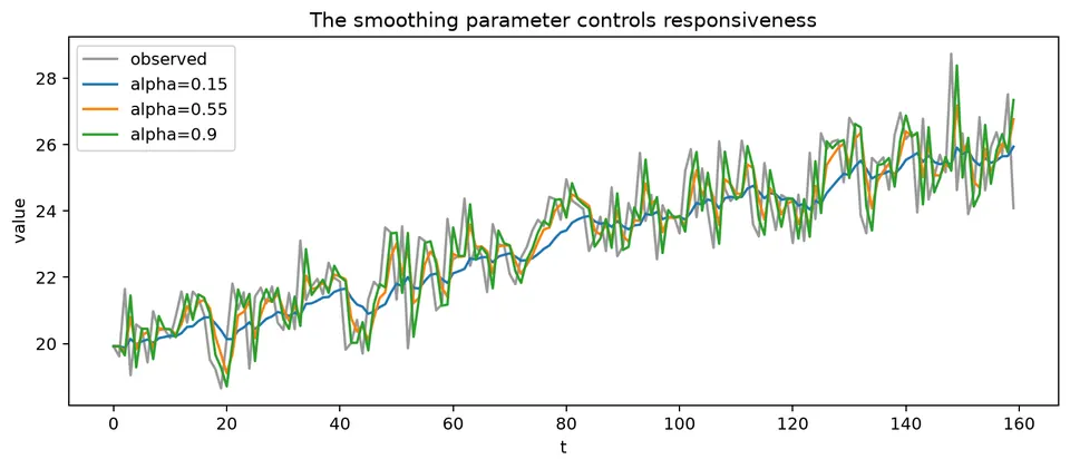
The figure shows how the smoothed level reacts to new observations. Higher responsiveness follows recent movements more closely but can also chase short-lived noise.

Initial Condition

A simple initialization is

$$ \ell_1=x_1. $$

The initialization contributes a term weighted by $(1-\alpha)^t$ after repeated updates. With a small $\alpha$, that weight can remain substantial for many observations, so the first value is not an innocuous choice in a short series. Estimating the initial level jointly with the smoothing parameter, or using an explicitly documented early-data estimate, makes the fitted procedure reproducible.

Forecast Error

The one-step forecast error is

$$ e_t=x_t-\hat x_{t\mid t-1}. $$

These errors can be used to choose the smoothing parameter and to diagnose whether a level-only model is adequate.

Sum of Squared Errors (SSE)

One fitting criterion is

$$ \mathrm{SSE}(\alpha)=\sum_t(x_t-\hat x_{t\mid t-1})^2. $$

A value of $\alpha$ can be selected by minimizing this criterion, although state-space formulations often estimate smoothing parameters and initial states jointly by likelihood.

Choosing the Optimal Smoothing Parameter

A value of $\alpha$ close to 1 gives most weight to recent data and adapts quickly. A value close to 0 changes slowly and averages information over a longer effective history.

Choose $\alpha$ from a fitting criterion or temporal validation rather than from visual smoothness alone. A smoother-looking fitted line is not necessarily a better forecast.

Recursive Form of SES

The recursive update

$$ \ell_t=\alpha x_t+(1-\alpha)\ell_{t-1} $$

requires only the previous state and the newest observation. This makes SES computationally efficient and naturally suited to sequential updating.

Holt’s Linear Trend Method (Double Exponential Smoothing)

Holt's method separates two evolving quantities: a level and a local slope. Before seeing the new observation, the previous slope advances the previous level by one step. The level update then compares that prediction with the observation, and the slope update revises the estimated rate of change. Keeping separate states prevents each short-term surprise from being interpreted as a permanent new trend.

$$ \ell_t=\alpha x_t+(1-\alpha)(\ell_{t-1}+b_{t-1}), $$

$$ b_t=\beta(\ell_t-\ell_{t-1})+(1-\beta)b_{t-1}, $$

with forecast

$$ \hat x_{t+h\mid t}=\ell_t+hb_t. $$

The level state estimates the current baseline, while $b_t$ estimates the local slope. Initial values can be set from the first observations or estimated jointly with the smoothing parameters.

The undamped forecast adds the same estimated slope at every future step, which can be unrealistic over long horizons. A damped trend progressively reduces those future slope contributions. Damping changes the extrapolation assumption, not just the appearance of the fitted trend, so compare it at the horizons where the forecasts will be used.

Holt-Winters Seasonal Method (Triple Exponential Smoothing)

Holt-Winters adds a seasonal state to level and trend. In the additive version, a seasonal state is measured in the response's units; an effect of 10 adds 10 at any level. In the multiplicative version, it is a factor; 1.10 means 10% above the underlying level. The multiplicative equations therefore need a meaningful positive scale and valid divisions, while additive equations can describe fixed seasonal shifts.

Additive Model

A common additive formulation is

$$ \ell_t =\alpha(x_t-s_{t-L}) +(1-\alpha)(\ell_{t-1}+b_{t-1}), $$

$$ b_t =\beta(\ell_t-\ell_{t-1}) +(1-\beta)b_{t-1}, $$

$$ s_t =\gamma(x_t-\ell_t) +(1-\gamma)s_{t-L}. $$

The $h$-step forecast is

$$ \hat x_{t+h\mid t} =\ell_t+hb_t+s_{t+h-L\lceil h/L\rceil}. $$

The seasonal index selects the most recent state for the corresponding future season. It cycles through the $L$ estimated seasonal positions as the horizon grows; it does not require an unobserved future seasonal state to be supplied as input.

Multiplicative Model

A common multiplicative formulation is

$$ \ell_t =\alpha\frac{x_t}{s_{t-L}} +(1-\alpha)(\ell_{t-1}+b_{t-1}), $$

$$ b_t =\beta(\ell_t-\ell_{t-1}) +(1-\beta)b_{t-1}, $$

$$ s_t =\gamma\frac{x_t}{\ell_t} +(1-\gamma)s_{t-L}, $$

with forecast

$$ \hat x_{t+h\mid t} =(\ell_t+hb_t)s_{t+h-L\lceil h/L\rceil}. $$

For additive seasonality, initial seasonal states are commonly centered to sum to zero. For multiplicative seasonality, they are commonly scaled to average 1. The exact initialization and state equations vary across software and ETS formulations, so reproduce the parameterization when comparing results.

Linear Prediction for Stationary Series

For a weakly stationary series with mean $\mu$, a linear predictor of $X_{n+h}$ based on $X_n,\ldots,X_1$ can be written as follows. The best linear predictor minimizes mean squared error within this linear class. It equals the full conditional mean under joint Gaussianity, but that equality does not follow from weak stationarity alone:

$$ \hat X_{n+h} =\mu+\sum_{i=1}^{n}a_i(X_{n+1-i}-\mu). $$

The coefficient vector solves the covariance system

$$ \Gamma_na=\gamma_n(h), $$

where $\Gamma_n$ is the Toeplitz covariance matrix of the predictors and $\gamma_n(h)$ is the covariance vector between the target and those predictors.

The corresponding linear-prediction mean squared error is

$$ \mathrm{MSE} =\gamma(0)-a^\top\gamma_n(h). $$

For a stationary Gaussian series and one predictor $X_n$,

$$ E(X_{n+h}\mid X_n) =\mu+\rho(h)(X_n-\mu). $$

For a centered AR(1), this reduces to

$$ \hat X_{n+h|n}=\phi^hX_n. $$

Algorithms such as Durbin-Levinson and the innovations algorithm exploit Toeplitz and innovations structure to compute predictors efficiently.

ARAR Algorithm

The ARAR algorithm uses an autoregressive prefilter to shorten strong persistence before fitting a lower-order dynamic model. A typical sequence is to filter the persistent series, fit an AR-type or ARMA-type model on the filtered representation, forecast there, and then invert the filter.

The method is useful as a historical forecasting approach for strongly persistent series. As with any transformation, the inverse step and forecast uncertainty must be carried back to the original scale consistently.

Machine Learning for Time Series Forecasting

Machine-learning methods can be useful when nonlinear interactions, many predictors, or large collections of related series are available. They are not inherently more accurate than statistical time-series models; performance depends on data volume, signal structure, feature availability, horizon, and the validation design.

A machine-learning row must reproduce what would have been known at its forecast origin. To predict $y_t$, a lag-1 feature is $y_{t-1}$, not $y_t$, and a rolling mean must end before the target becomes available. For a longer horizon, some values available to a one-step row become future information. Construct features from the horizon and information timing, then choose the prediction algorithm.

Key Challenges in Time Series Forecasting

Machine-learning forecasting must handle temporal dependence, evolving distributions, seasonality and trend, multi-step prediction, and the possibility of leakage through feature construction or preprocessing.

Many generic ML algorithms do not contain a built-in concept of time. The time-series structure enters through the feature design, target construction, recursive/direct forecasting strategy, and chronological evaluation.

Supervised Learning Approach for Time Series

A forecasting problem can be converted into supervised rows. To predict $y_t$, features might include

$$ y_{t-1},y_{t-2},\ldots, $$

along with lagged external variables, calendar indicators, and trailing-window summaries.

Data Preparation (Feature Engineering for Time Series)

Useful features include lagged values, trailing-window means or variances, calendar variables, known future events, and external predictors. All rolling features should be trailing or otherwise explicitly past-only in a real-time forecast.

The target horizon must also be explicit. A feature table for one-step forecasting is not automatically valid for forecasting 12 steps ahead.

Machine Learning Models for Time Series Forecasting

Tree ensembles, boosting models, support-vector regression, and feed-forward neural networks can all be applied after the forecasting problem has been transformed into a supervised dataset.

A random forest maps one supplied feature row to a prediction. It does not automatically generate the lagged values needed several steps into the future. A recursive strategy feeds earlier predictions into later feature rows; a direct strategy fits a separate target horizon; a multi-output strategy predicts several horizons together. These are distinct forecasting procedures even when they use the same underlying tree algorithm.

from sklearn.ensemble import RandomForestRegressor

# 'data' contains a time-ordered target column named 'value'.
data['lag1'] = data['value'].shift(1)
data['lag2'] = data['value'].shift(2)
data = data.dropna()

# Chronological split.
train_size = int(len(data) * 0.8)
train = data.iloc[:train_size]
test = data.iloc[train_size:]

X_train = train[['lag1', 'lag2']]
y_train = train['value']
X_test = test[['lag1', 'lag2']]

rf_model = RandomForestRegressor(n_estimators=100)
rf_model.fit(X_train, y_train)
predictions = rf_model.predict(X_test)

The chronological split keeps training targets earlier than test targets. In this one-step example, a test row can use the previous realized observation once that value has actually arrived. Forecasting the entire test block from one initial origin would require a different feature construction or recursive strategy. Repeat the procedure over several origins when assessing how it would perform through time.

Gradient Boosting Machines (GBM, XGBoost, LightGBM, CatBoost)

Gradient boosting builds trees sequentially so that later trees reduce errors left by earlier ones. It can model nonlinear interactions in structured lag-feature datasets and often performs well when there are many informative covariates.

Boosted trees divide the feature space into fitted regions rather than extending a learned linear slope indefinitely. A strong trend that carries future values beyond the training range can therefore be difficult to extrapolate. Lag features, transformations, and a separate trend component may help, but they must be fitted inside the historical training boundary. Evaluate their contribution rather than attributing success or failure to the model family name alone.

import xgboost as xgb

xgb_model = xgb.XGBRegressor(
    n_estimators=100,
    max_depth=3,
    learning_rate=0.1,
)
xgb_model.fit(X_train, y_train)
predictions = xgb_model.predict(X_test)

Support Vector Machines (SVM)

Support Vector Regression (SVR) can learn nonlinear relationships through kernels such as the radial basis function. It is sensitive to feature scaling and can become computationally expensive as the training sample grows.

from sklearn.svm import SVR

svr_model = SVR(kernel='rbf', C=100, gamma=0.1)
svr_model.fit(X_train, y_train)
predictions = svr_model.predict(X_test)

Artificial Neural Networks (ANN)

A feed-forward neural network can map lagged and external features to future targets. Its flexibility can capture nonlinear relationships, but it also increases data requirements and overfitting risk.

from sklearn.neural_network import MLPRegressor

mlp_model = MLPRegressor(
    hidden_layer_sizes=(100,),
    activation='relu',
    solver='adam',
    max_iter=1000,
)
mlp_model.fit(X_train, y_train)
predictions = mlp_model.predict(X_test)

Advanced Neural Network Models for Time Series

A recurrent network updates an internal state as observations arrive. That state can represent information distributed across several earlier dates, reducing the need to supply every lag as a separate flat feature. Training must still decide how long sequences are, how the state is initialized or carried across batches, and which observations are available at prediction time. Sequential architecture does not itself prevent leakage or make a short dataset informative enough for a large model.

Recurrent Neural Networks (RNNs)

A simple RNN passes a hidden state from one time step to the next. Standard RNNs can struggle with long dependencies because gradients may vanish or explode.

import tensorflow as tf

model = tf.keras.models.Sequential([
    tf.keras.layers.SimpleRNN(
        50,
        activation='relu',
        input_shape=(n_timesteps, n_features),
    ),
    tf.keras.layers.Dense(1),
])

model.compile(optimizer='adam', loss='mse')
model.fit(X_train, y_train, epochs=50, batch_size=32)

Long Short-Term Memory (LSTM)

LSTMs introduce gated memory cells that improve gradient flow over longer sequences. They can model nonlinear temporal patterns, but they require careful regularization, scaling, architecture selection, and chronological evaluation.

import tensorflow as tf

X_train_reshaped = X_train.values.reshape(
    (X_train.shape[0], X_train.shape[1], 1)
)
X_test_reshaped = X_test.values.reshape(
    (X_test.shape[0], X_test.shape[1], 1)
)

model = tf.keras.models.Sequential([
    tf.keras.layers.LSTM(
        50,
        activation='relu',
        input_shape=(X_train_reshaped.shape[1], X_train_reshaped.shape[2]),
    ),
    tf.keras.layers.Dense(1),
])

model.compile(optimizer='adam', loss='mse')
model.fit(X_train_reshaped, y_train, epochs=100, batch_size=32)
predictions = model.predict(X_test_reshaped)

Gated Recurrent Units (GRU)

GRUs use a simpler gating structure than LSTMs and can provide similar performance with fewer parameters in some problems. Neither architecture is universally preferable; the comparison should be made on chronological validation data.

import tensorflow as tf

model = tf.keras.models.Sequential([
    tf.keras.layers.GRU(
        50,
        activation='relu',
        input_shape=(n_timesteps, n_features),
    ),
    tf.keras.layers.Dense(1),
])

model.compile(optimizer='adam', loss='mse')
model.fit(X_train, y_train, epochs=50, batch_size=32)

Hybrid Models

A hybrid can first fit a linear dynamic model and then fit a nonlinear model to what remains. The second stage should learn residual structure that is reproducible beyond the training sample, not simply fit the noise left by the first stage. Train both stages within each forecast origin and compare the combined forecasts with each component separately. Otherwise any apparent improvement may come from extra fitting opportunities rather than a useful complementary mechanism.

Each stage should be trained inside the same historical information boundary, and the hybrid should be compared with its simpler components on identical forecast origins.

Comparison of Various Models

The table below summarizes common forecasting families. The descriptions are broad; implementations within each family differ substantially.

Model structure and use

Strengths and limitations

Compare the families on the same forecasting task: target, forecast origins, horizons, available predictors, and evaluation scale. Accuracy and calibration measure predictive behavior, while complexity and interpretability determine whether the method is practical to fit, explain, maintain, and update.

Model Evaluation

Forecast accuracy must be evaluated out of sample with temporal order preserved. Point-forecast metrics summarize different loss functions:

AIC and BIC are not forecast-error metrics. They compare likelihood-based candidate models fitted to the same response data:

$$ \mathrm{AIC}=2k-2\log L, $$

$$ \mathrm{BIC}=k\log n-2\log L. $$

Residual tests such as Ljung-Box are diagnostics rather than accuracy scores. They assess whether a fitted model has left linear autocorrelation unexplained.

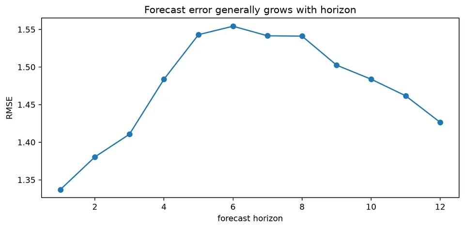
The horizon plot shows why a single average metric can be misleading. A method that is strongest one step ahead may lose its advantage at longer horizons, so evaluation should match the operational forecast horizon.

Forecast targets, transformations, and uncertainty

A forecast is a conditional statement. Under squared-error loss,

$$ \hat y_{T+h\mid T}=E(y_{T+h}\mid\mathcal F_T). $$

The conditioning set $\mathcal F_T$ is as important as the model family. A forecast that uses a realized future predictor answers a different question from one that uses only information available in deployment.

Baselines first

For a level series, the naive forecast is

$$ \hat y_{T+h\mid T}=y_T. $$

For seasonal period $s$, the seasonal-naive rule reuses the latest observation from the same season. A drift forecast extrapolates the historical average change. Report at least one appropriate baseline before presenting ARIMA, state-space, or machine-learning results.

Simple exponential smoothing

For a roughly level series,

$$ \ell_t=\alpha y_t+(1-\alpha)\ell_{t-1}, \qquad \hat y_{t+h\mid t}=\ell_t. $$

If $\ell_{t-1}=100$, $y_t=110$, and $\alpha=0.3$,

$$ \ell_t=0.3(110)+0.7(100)=103. $$

Under the level-only model, the forecast is 103 for every future horizon. Increasing $\alpha$ makes the level respond faster to recent observations but can also make it more sensitive to noise.

Holt trend and seasonal extensions

Holt's linear trend keeps a level and slope:

$$ \ell_t=\alpha y_t+(1-\alpha)(\ell_{t-1}+b_{t-1}), $$

$$ b_t=\beta(\ell_t-\ell_{t-1})+(1-\beta)b_{t-1}, $$

with

$$ \hat y_{t+h\mid t}=\ell_t+hb_t. $$

Holt-Winters adds a seasonal state. The additive version keeps seasonal amplitude in the response units; the multiplicative version lets it scale with the level.

AR forecast example

For

$$ y_t=0.8y_{t-1}+\varepsilon_t, \qquad y_T=5, $$

the one-step and five-step forecasts are

$$ \hat y_{T+1|T}=4, \qquad \hat y_{T+5|T}=0.8^5(5)=1.6384. $$

With innovation variance 1, the two-step forecast-error variance is

$$ 1+0.8^2=1.64. $$

An approximate 95% Gaussian interval around the two-step mean $3.2$ is

$$ 3.2\pm1.96\sqrt{1.64}. $$

The point forecast shrinks toward the mean while uncertainty increases.

Forecast transformations

If a model forecasts $\log y_t$, then

$$ \exp(E[\log y_t\mid\mathcal F_T]) $$

is generally not the conditional mean of $y_t$. Jensen's inequality gives

$$ E[\exp(Z)]\ne\exp(E[Z]). $$

For a conditional normal distribution on the log scale with mean $m$ and variance $v$, the original-scale median is $e^m$, while the mean is $e^{m+v/2}$. The difference grows with uncertainty because exponentiation stretches the upper tail more than the lower tail. Transform interval endpoints consistently, and state which point target is being reported; exponentiating a log-scale mean does not automatically give an original-scale mean forecast.

Forecast combination

Two forecasts can be combined as

$$ \hat y=w\hat y^{(1)}+(1-w)\hat y^{(2)}. $$

Combining helps when the errors are complementary: one forecast can offset misses made by the other. If both make almost identical errors, averaging them adds little. The weight therefore belongs to model development and must be chosen from training or validation origins. Evaluating many weights on the final test period turns that period into tuning data and invalidates its role as an independent assessment.

Forecast uncertainty

Forecast uncertainty can come from future shocks, parameter estimation, future predictor values, transformation bias, model uncertainty, and regime changes. Classical model intervals may include only a subset of these sources.

The widening intervals reinforce the distinction between point prediction and uncertainty. Evaluate empirical coverage and width on temporal backtests, and state which uncertainty sources the interval construction includes.

Communication

A useful forecast report includes:

1. forecast origin and timestamp;
2. horizon and units;
3. point forecast and target functional;
4. interval level and construction;
5. baseline comparison;
6. recent error history;
7. known future events or predictor assumptions;
8. limitations and update schedule.

Formula reference