Statistical hypothesis testing is a method for using sample data to make inferences about a population. Understanding null and alternative hypotheses, along with how p-values are calculated and interpreted, is essential for applying hypothesis tests correctly.

After reading this material, you should be able to explain:

• What a null hypothesis is and how it relates to the p-value
• How to calculate a p-value
• How to interpret a p-value

What is Null Hypothesis?

In statistical hypothesis testing, we define two competing hypotheses about a population parameter:

1. The null hypothesis ($H_0$) specifies the claim being tested. It often represents no effect, no difference, or no change, although more generally it specifies a particular value or model. For example, when testing a new drug, the null hypothesis might state that the drug has the same average effect as a placebo.
2. The alternative hypothesis ($H_1$ or $H_a$) describes the competing claim. In the drug example, it might state that the drug and placebo have different effects.

Choosing appropriate hypotheses depends on the research question. The null hypothesis usually provides a precise benchmark against which the observed data can be evaluated, while the alternative describes the departure from that benchmark that is scientifically relevant.

The relationship between the null and alternative hypotheses is central to null hypothesis significance testing (NHST), which is widely used in fields such as medicine, psychology, neuroscience, genetics, economics, and linguistics.

The basic goal of NHST is to use sample data to assess whether there is sufficient evidence to reject the null hypothesis in favor of the alternative. This decision is based on the p-value, which measures how unusual the observed result would be if the null hypothesis were true.

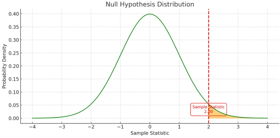
The plot illustrates the distribution of a test statistic under the assumption that the null hypothesis $H_0$ is true:

• The green curve (null distribution) represents the probability distribution of the test statistic under $H_0$. Its exact form depends on the statistical test being used, such as a normal or t-distribution.
• The vertical dashed red line marks the observed value of the test statistic calculated from the sample data.
• The orange shaded area (tail area) represents the probability of obtaining a test statistic at least as extreme as the observed value under $H_0$. This area is the p-value. In a one-tailed test, only the relevant tail is considered. In a two-tailed test, extreme outcomes in both directions are included.

The Language of Hypothesis Testing

• If the evidence is strong enough, typically when $p < \alpha$, we reject $H_0$, indicating statistically significant evidence in favor of the alternative hypothesis.
• When the evidence is insufficient, we fail to reject $H_0$. This does not mean that $H_0$ has been shown to be true; it means that the data do not provide enough evidence against it.
• We generally avoid saying that we accept $H_0$, because a hypothesis test is designed to assess evidence against $H_0$, not to prove it.
• A Type I error occurs when we reject $H_0$ even though it is true.
• A Type II error occurs when we fail to reject $H_0$ even though the alternative is true.

Understanding P-Values Through an Analogy

Imagine that you are a detective evaluating evidence against a suspect. In this analogy, the null hypothesis ($H_0$) is that the suspect is innocent, while the alternative hypothesis ($H_a$) is that the suspect is guilty.

As you collect evidence—such as fingerprints, DNA samples, or eyewitness accounts—you ask how unusual evidence this strong would be if the suspect were innocent.

The p-value plays a similar role: it measures how unusual the observed result, or a more extreme one, would be under the assumption that $H_0$ is true.

In a one-tailed test, only evidence in a specified direction is treated as evidence against $H_0$. In a two-tailed test, extreme results in either direction are considered.

If the p-value is small, for example below a significance level of 5%, the observed evidence would be unusual under $H_0$. In statistical testing, this leads us to reject $H_0$.

A large p-value means the evidence is not sufficiently unusual under $H_0$, so we fail to reject it.

The analogy has an important limitation: a p-value is not the probability that the suspect is innocent or guilty. Likewise, in statistical testing it is not the probability that $H_0$ is true or false.

Interpretation of the P-value

The p-value is the probability of obtaining a test statistic at least as extreme as the one observed, assuming that the null hypothesis $H_0$ is true.

• The p-value does not represent the probability that $H_0$ is true or false.
• A large p-value means that the observed result is reasonably compatible with $H_0$, but it does not prove that $H_0$ is true.
• A small p-value ($p < \alpha$) provides evidence against $H_0$, leading us to reject the null hypothesis.
• A large p-value ($p \geq \alpha$) indicates insufficient evidence to reject $H_0$, so we fail to reject it.

Example: Coin Toss Experiment

• The null hypothesis ($H_0$) states that the coin is fair:

$$ P(\text{heads}) = 0.5 $$

• The alternative hypothesis ($H_1$) states that the coin is not fair:

$$ P(\text{heads}) \neq 0.5 $$

• The experiment involves 10 tosses ($n = 10$).
• The observed outcome is 4 heads and 6 tails.

Statistical Test

We use a binomial test to calculate the p-value.

I. Compute the probability of observing exactly 4 heads under $H_0$:

$$ P(X = 4) = \binom{10}{4}(0.5)^4(0.5)^6 = 210(0.5)^{10} \approx 0.2051 $$

II. Compute the probabilities of outcomes at least as extreme as the observed result.

Because this is a two-tailed test with a fair coin, outcomes of 0 to 4 heads and 6 to 10 heads are equally or more extreme than the observed result.

III. Total P-value:

By symmetry:

$$ \text{p-value} = 2P(X\leq4) = 2\left(\sum_{k=0}^{4}P(X=k)\right) $$

IV. Sum of Probabilities:

$$ \begin{align} P(X = 0) &= 0.00098 \\ P(X = 1) &= 0.00977 \\ P(X = 2) &= 0.04395 \\ P(X = 3) &= 0.11719 \\ P(X = 4) &= 0.20508 \\ \sum_{k=0}^{4} P(X = k) &= 0.37697 \end{align} $$

V. Compute P-value:

$$ \text{p-value} = 2(0.37697) = 0.75394 $$

Decision

• The significance level ($\alpha$) is set at 0.05.
• The p-value is $0.75394$, which is greater than $0.05$.
• Therefore, we fail to reject $H_0$.
• The data do not provide sufficient evidence to conclude that the coin is unfair.

This does not mean that we have proved the coin is fair. It only means that the observed result is consistent with what we could reasonably see from a fair coin.

Additional Considerations

• Statistical power is the probability of correctly rejecting $H_0$ when the alternative hypothesis is true.
• Sample size affects power; all else being equal, larger samples generally provide greater power.
• A one-tailed test examines an effect in one specified direction, such as $P(\text{heads}) > 0.5$.
• A two-tailed test examines departures in either direction, such as $P(\text{heads}) \neq 0.5$.
• Confidence intervals provide a range of plausible values for a population parameter based on sample data.
• For many standard two-sided tests, if the corresponding confidence interval does not contain the null value, $H_0$ is rejected at the matching significance level.