Central Limit Theorem (CLT)
The central limit theorem describes the fluctuations of a sum or average around its expectation. For independent, identically distributed observations with finite, positive variance, the centered and standardized mean approaches a standard normal distribution as sample size grows. The population can remain skewed or discrete throughout: it is the distribution of the statistic across repeated samples that is approximated.
Mathematical Background
Suppose a population has mean $\mu$ and standard deviation $\sigma$. If we repeatedly take sufficiently large random samples of size $n$, then the distribution of the sample means is approximately normal under the usual CLT assumptions.
The sampling distribution of the mean has:
I. Mean equal to the population mean (this holds exactly for every $n$, not only approximately):
$$ E[\bar{X}] = \mu $$
II. Standard deviation, called the standard error:
$$ SE(\bar{X}) = \frac{\sigma}{\sqrt{n}} $$
As $n$ increases, the standard error decreases, so sample means become more tightly concentrated around $\mu$.
Formal Description
Let $X_1, X_2, \ldots, X_n$ be independent and identically distributed random variables, each with mean $\mu$ and variance $0<\sigma^2<\infty$. Centering a sum subtracts $n\mu$, and dividing by its standard deviation $\sigma\sqrt n$ produces a dimensionless quantity with variance one.
As $n$ tends to infinity, the standardized sum
$$ \frac{X_1 + X_2 + \cdots + X_n - n\mu}{\sigma\sqrt{n}} $$
converges in distribution to a standard normal distribution. Equivalently,
$$ P\left( \frac{X_1 + X_2 + \cdots + X_n - n\mu} {\sigma\sqrt{n}} \leq a \right) \to \frac{1}{\sqrt{2\pi}} \int_{-\infty}^{a} e^{-x^2/2}dx $$
Important points:
- There is no universal cutoff such as 30 observations. Approximation error depends on the population distribution and the probability being calculated.
- The sampled observations should be independent.
- The theorem applies to the distribution of sample means, sums, and some related statistics. It does not make the individual observations normally distributed.
- Strongly skewed or heavy-tailed populations may require much larger samples before the normal approximation becomes accurate.
Why Centered Sums Approach a Common Shape
Centering removes the population location, and scaling removes its variance. Let $W_i=(X_i-\mu)/\sigma$, so $E[W_i]=0$ and $E[W_i^2]=1$. The standardized mean is $Z_n=n^{-1/2}\sum_iW_i$. For a finite-variance variable, its characteristic function $\phi_W(t)=E[e^{itW}]$ satisfies
$$ \phi_W(t)=1-\frac{t^2}{2}+o(t^2) \quad\text{as }t\to0. $$
The linear term vanishes because the mean is zero, and the quadratic term is determined by the variance. Independence makes the characteristic function of the sum a product:
$$ \phi_{Z_n}(t) =\left[\phi_W\left(\frac{t}{\sqrt n}\right)\right]^n =\left[1-\frac{t^2}{2n}+o\left(\frac1n\right)\right]^n \longrightarrow e^{-t^2/2}. $$
The limit is the standard normal characteristic function. A characteristic-function convergence theorem then gives convergence in distribution. This argument explains the common shape: after centering and scaling, the second-order behavior is shared, while the remaining terms vanish in this limit. It does not require the population to have an MGF, which may fail to exist even when its variance is finite.
The theorem concerns the cumulative probabilities of $Z_n$ at fixed thresholds. It supplies a limiting statement rather than a specified error at a particular n. Approximating an extremely small tail probability can require more care than approximating a central probability, because a small absolute error can be a large fraction of a tiny probability.
Replacing the Population Standard Deviation
For i.i.d. observations with finite positive variance, the sample variance is consistent: $S_n^2\to\sigma^2$ in probability. This follows from the law of large numbers applied to $X_i^2$, together with convergence of $\bar X_n$. Hence
$$ \frac{\sqrt n(\bar X_n-\mu)}{S_n} =\frac{\sqrt n(\bar X_n-\mu)}{\sigma} \frac{\sigma}{S_n} \ \xrightarrow{d}\ N(0,1). $$
The second factor tends to one, so it does not change the limiting distribution. This is an application of Slutsky's theorem. It explains a large-sample justification for estimating the standard error; it does not make the finite-sample statistic exactly t distributed for a nonnormal population. The exact t result uses additional normal-sample independence.
Implications and Applications
The CLT allows probabilities involving large samples to be approximated with the normal distribution. This is central to statistical inference.
For example, suppose an online game has a 20% probability of awarding a small prize on each independent attempt. The number of wins follows a binomial distribution. When the number of attempts is large, that binomial distribution can often be approximated by a normal distribution, which simplifies probability calculations.
The CLT is useful because:
- It applies to many population distributions when the sample size is sufficiently large.
- It gives approximate probabilities and error margins for estimates computed from sample statistics.
- It supports confidence intervals and hypothesis tests.
- It makes many otherwise difficult probability calculations manageable.
- It underlies a large number of statistical methods used in science, engineering, economics, and data analysis.
Limitations
The theorem depends on several conditions:
- The sample size must be large enough for the population being studied. There is no universal cutoff that works for every distribution.
- Observations should be independent.
- The classical CLT assumes that the population has a finite variance.
- Severe skewness, extreme outliers, or heavy tails can make convergence to normality slow.
- Dependence between observations can invalidate the standard form of the theorem.
An Exponential Example with an Exact Answer
Let $X_i$ be independent exponential observations with rate one. They have mean one, variance one, and a strongly right-skewed distribution. Their sum has a Gamma distribution with shape n and rate one, so the average has a Gamma distribution with shape n and rate n:
$$ \bar X_n\sim\mathrm{Gamma}(n,\text{rate }n). $$
This exact distribution has mean one, variance $1/n$, and skewness $2/\sqrt n$. The CLT approximates $\sqrt n(\bar X_n-1)$ by a standard normal variable. The table compares one exact probability with the normal prediction:
| Sample size n | Exact skewness of the mean | Exact $P(\bar X_n\leq1)$ | CLT approximation |
|---|---|---|---|
| 1 | 2.0 | 0.6321 | 0.5000 |
| 4 | 1.0 | 0.5665 | 0.5000 |
| 25 | 0.4 | 0.5266 | 0.5000 |
| 100 | 0.2 | 0.5133 | 0.5000 |
The approximation is one half because one is the population mean, corresponding to standardized threshold zero. The exact probabilities approach that value as the right skew diminishes. This calculation shows both progress toward normality and the remaining asymmetry at finite sample sizes.
The absolute spread also decreases: the standard deviations of these means are 1, 0.5, 0.2, and 0.1. Concentration and shape improvement occur together here, but they are distinct mathematical claims. A simulation can reproduce the exact Gamma distributions; increasing the number of simulation repetitions cannot remove their finite-n skewness.
Discrete Counts and Continuity Correction
For $K\sim\mathrm{Binomial}(n,p)$, the mean and variance are $np$ and $np(1-p)$. The CLT motivates a normal approximation when the binomial distribution is sufficiently well spread. Because K is integer valued, the event $45\leq K\leq55$ includes all the probability mass at both endpoints.
For 100 fair trials, the normal approximation has mean 50 and standard deviation five. Moving the continuous boundaries half a count outward gives
$$ P(45\leq K\leq55) \approx \Phi\left(\frac{55.5-50}{5}\right) -\Phi\left(\frac{44.5-50}{5}\right) \approx0.7287. $$
The exact binomial probability is about 0.72875. Using the boundaries 45 and 55 without correction gives about 0.68269, omitting the half-width contribution at each endpoint. The continuity correction matches the continuous interval to the integer cells being counted. It improves this example substantially, but it is not a replacement for checking whether the underlying normal approximation is appropriate.
For contrast, take $n=30$ and $p=0.01$. The expected count is 0.3, the variance is 0.297, and $P(K=0)=0.99^{30}\approx0.7397$. A normal distribution with the same mean and variance assigns about 0.291 of its probability to values below zero, which are impossible for K. Thirty trials have not created a symmetric count distribution.
The standardized third absolute moment helps explain why rare events need larger n. When it exists, a Berry–Esseen bound controls the maximum absolute CDF error by a universal constant times $E[|X-\mu|^3]/(\sigma^3\sqrt n)$. A large standardized third moment can offset the apparent advantage of a moderately large n. The classical finite-variance CLT does not itself require this third moment; the bound is a stronger result with a stronger assumption.
Visualization
The sample size and the number of simulation repetitions have different roles. Increasing the size $n$ of each sample can improve the normal approximation predicted by the CLT. Increasing the number of repeated samples merely makes the histogram a more accurate picture of the sampling distribution for that fixed $n$. One million simulated means of samples of size one would still display the original population distribution, rather than make it normal.
Data Generation
In this example:
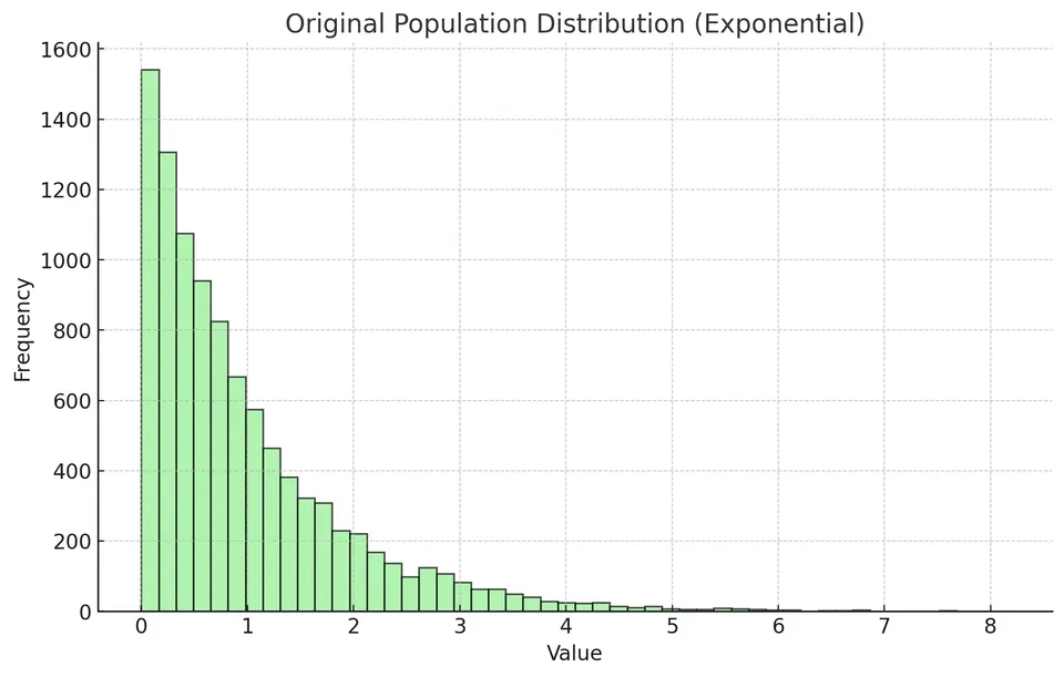
- The population is generated from a non-normal exponential distribution.
- The exponential distribution has scale parameter $1.0$.
- The population contains 10,000 observations.
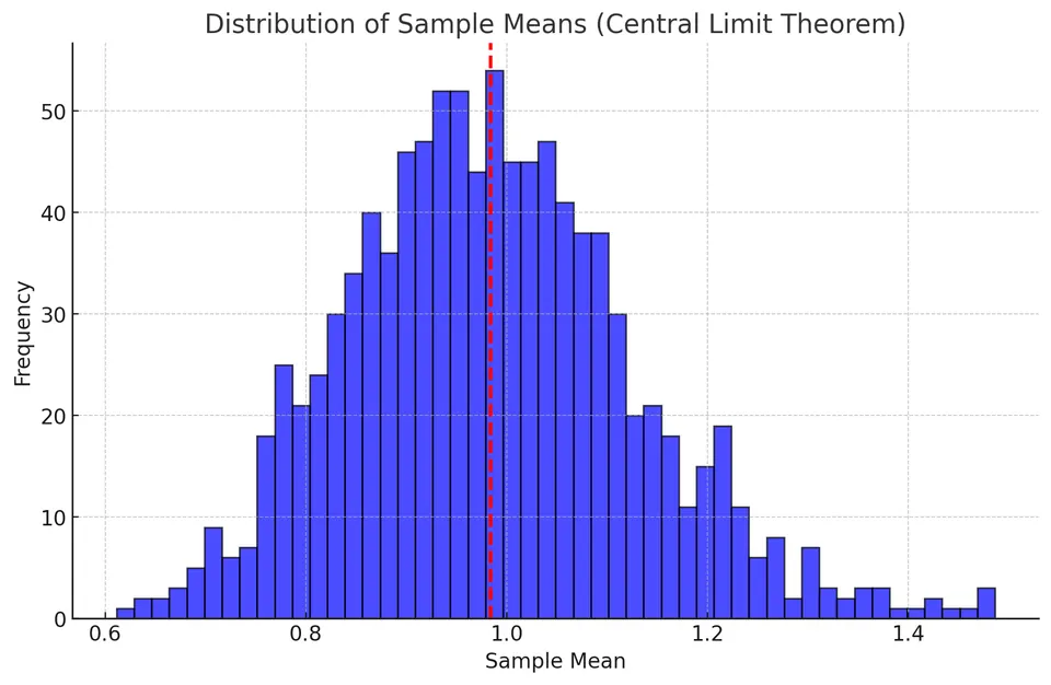
- We draw 1,000 samples.
- Each sample contains 50 observations.
The plot below shows the original exponential population, which is strongly right-skewed.
Distribution of Sample Means
For each of the 1,000 samples, the sample mean is calculated using
$$ \bar{x} = \frac{1}{n}\sum_{i=1}^{n}x_i $$
where:
- $\bar{x}$ is the sample mean;
- $n$ is the sample size;
- $x_i$ is the $i$-th observation in the sample.
The second plot shows the distribution of those sample means. The distribution is approximately bell-shaped even though the original population is not normal.
Results from the simulation:
- Mean of the generated 10,000-value population: approximately $0.9775$.
- Mean of the sample means: approximately $0.9843$.
- Standard deviation of the sample means (empirical standard error): approximately $0.1378$, versus $1/\sqrt{50}\approx0.1414$ for independent draws from the underlying rate-one exponential law.
- The sample means form an approximately normal distribution.
The underlying exponential law has mean one. The generated finite population has its own realized mean and variance. If each sample is drawn with replacement from that fixed population, its conditional mean and standard error use those finite-population quantities; without replacement, a finite population correction also applies. Drawing directly from the exponential law instead uses mean and variance one. The mean of repeated sample means is close to the relevant expectation, as expected from $E[\bar X]=\mu$ (this part does not need the CLT). The bell shape of the histogram is the CLT's contribution. The observed spread is also consistent with the standard-error formula
$$ SE(\bar{X}) = \frac{\sigma}{\sqrt{n}} $$
Concentration and distributional shape are separate claims
The law of large numbers gives $\bar X\to\mu$ under suitable conditions. The CLT refines the picture by studying $\sqrt n(\bar X-\mu)$ rather than the shrinking unscaled difference. Its scale factor prevents the limiting distribution from collapsing to a point. For the exponential model with mean and standard deviation both equal to one, $\bar X$ has variance $1/n$, while $\sqrt n(\bar X-1)$ has variance one and becomes approximately standard normal.
Some distributions have a finite mean but infinite variance; the usual LLN can hold while this classical CLT fails. A Cauchy population lacks even a finite mean, and averaging independent Cauchy observations does not yield the concentration described here. These examples explain why checking moment conditions is more useful than relying on a universal sample-size cutoff.
A Finite Mean Does Not Imply a Finite Standard Error
A Pareto distribution with lower endpoint one and tail probability $P(X>x)=x^{-3/2}$ for $x\geq1$ has mean three but infinite variance. Independent averages satisfy a law of large numbers because the absolute mean is finite. The classical normalization by a finite $\sigma\sqrt n$ is unavailable, however, and the usual finite-variance CLT does not apply.
This separates two failures that can otherwise be confused. An i.i.d. Cauchy sample has no finite absolute mean, and its average has the same Cauchy distribution at every n. For that population, averaging does not even yield the concentration described by the usual LLN. A population with finite mean but infinite variance can concentrate while having different fluctuation scales and limits.
Dependence is another issue. If $X_i=U$ for every i, the mean is U regardless of sample size. More general CLTs can handle particular dependence structures, but they require additional assumptions and usually a variance including covariance contributions. The independent-sample formula is not justified by a large row count alone.
Standardizing Using the CLT
A sample statistic can be standardized with a z-score:
$$ z = \frac{\text{statistic} - \text{expected value}} {\text{standard error of the statistic}} $$
For a sample mean, this becomes
$$ z = \frac{\bar{x} - \mu}{SE(\bar{X})} = \frac{\bar{x} - \mu}{\sigma/\sqrt{n}} $$
The z-score tells us how many standard errors the observed sample mean lies above or below the population mean.
Step-by-Step Example
Suppose incomes have the following population parameters:
- Population mean: $\mu = 67{,}000$.
- Population standard deviation: $\sigma = 38{,}000$.
- Sample size: $n$.
Step 1: Calculate the Standard Error
The standard error of the sample mean is
$$ SE(\bar{X}) = \frac{\sigma}{\sqrt{n}} $$
For $n = 100$,
$$ SE(\bar{X}) = \frac{38{,}000}{\sqrt{100}} = \frac{38{,}000}{10} = 3{,}800 $$
Step 2: Calculate the z-score
Suppose the observed sample mean is $\bar{x} = 70{,}000$. Then
$$ z = \frac{70{,}000 - 67{,}000}{3{,}800} = \frac{3{,}000}{3{,}800} \approx 0.79 $$
The sample mean is approximately $0.79$ standard errors above the population mean.
Example: Applying the CLT
Suppose independent heights from a plant species follow a normal distribution with the parameters below. The sample mean is then exactly normal for every $n$, since linear combinations of independent normal variables are normal. This provides a reference calculation; the final case explains what changes when the population distribution is unknown:
- Population mean: $\mu = 15$ cm.
- Population standard deviation: $\sigma = 3$ cm.
- Sample size: $n$.
The standard error of the sample mean is
$$ SE(\bar{X}) = \frac{\sigma}{\sqrt{n}} $$
The z-score for a possible sample mean $x$ is
$$ z = \frac{x-\mu}{SE(\bar{X})} $$
We want to calculate
$$ P(14 \leq \bar{X} \leq 16) $$
for several sample sizes.
Sample Size of 16 Plants
For $n=16$,
$$ SE(\bar{X}) = \frac{3}{\sqrt{16}} = \frac{3}{4} = 0.75 $$
The z-score for $14$ cm is
$$ z_{14} = \frac{14-15}{0.75} = \frac{-1}{0.75} \approx -1.33 $$
The z-score for $16$ cm is
$$ z_{16} = \frac{16-15}{0.75} = \frac{1}{0.75} \approx 1.33 $$
Using the standard normal distribution,
$$ P(Z \leq -1.33) \approx 0.0918 $$
and
$$ P(Z \leq 1.33) \approx 0.9082 $$
Therefore,
$$ P(14 \leq \bar{X} \leq 16) = 0.9082 - 0.0918 = 0.8164 $$
The probability is approximately 81.64% (using the rounded $z=\pm1.33$; the unrounded $z=\pm1.3333$ gives 81.76%).
Sample Size of 64 Plants
For $n=64$,
$$ SE(\bar{X}) = \frac{3}{\sqrt{64}} = \frac{3}{8} = 0.375 $$
The corresponding z-scores are
$$ z_{14} = \frac{14-15}{0.375} \approx -2.67 $$
and
$$ z_{16} = \frac{16-15}{0.375} \approx 2.67 $$
Using the standard normal distribution,
$$ P(Z \leq -2.67) \approx 0.0038 $$
and
$$ P(Z \leq 2.67) \approx 0.9962 $$
Therefore,
$$ P(14 \leq \bar{X} \leq 16) = 0.9962 - 0.0038 = 0.9924 $$
The probability is approximately 99.24%.
Sample Size of 144 Plants
For $n=144$,
$$ SE(\bar{X}) = \frac{3}{\sqrt{144}} = \frac{3}{12} = 0.25 $$
The corresponding z-scores are
$$ z_{14} = \frac{14-15}{0.25} = -4 $$
and
$$ z_{16} = \frac{16-15}{0.25} = 4 $$
Using the standard normal distribution,
$$ P(Z \leq -4) \approx 0.00003 $$
and
$$ P(Z \leq 4) \approx 0.99997 $$
Therefore,
$$ P(14 \leq \bar{X} \leq 16) = 0.99997 - 0.00003 = 0.99994 $$
The probability is approximately 99.99%.
As the sample size increases, the standard error decreases. This makes the sample mean more concentrated around the population mean.
Unknown Population Distribution
Suppose the distribution of plant heights is unknown.
The CLT still allows the sampling distribution of the mean to be approximated by a normal distribution when the sample size is sufficiently large and the observations satisfy the theorem's assumptions.
For $n=64$, the calculations above may still be used as an approximation. The estimated probability remains approximately 99.24%, although the quality of the approximation depends on the actual shape of the population distribution.