Spatial Validation

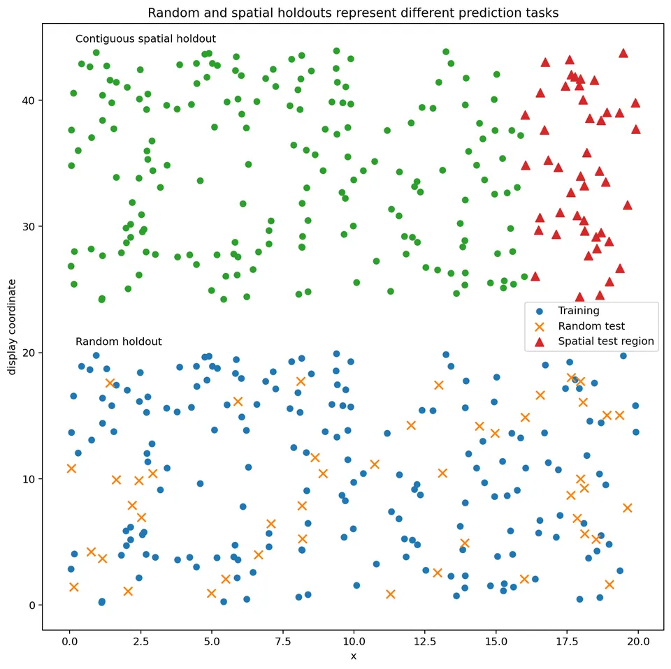
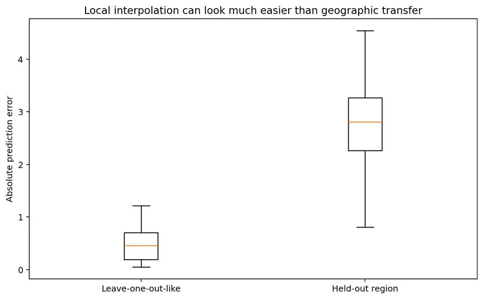
Spatial model performance depends not only on which observations are held out, but also on where those observations are located relative to the training data. This makes spatial validation fundamentally different from ordinary random train/test splitting. A random split often leaves test locations surrounded by nearby training observations, so it evaluates an interpolation-like task. A geographically separated holdout removes some nearby information and often asks a harder prediction question. The actual difficulty also depends on the covariates, sampling density, and training size. Its target is:

Can the model predict where nearby observations are unavailable?

Neither design is universally correct. The appropriate validation design is the one that best reproduces the information conditions expected at deployment.

A Validation Score Estimates a Particular Prediction Risk

Let D denote the information available to fit a predictor $\hat f_D$. Let Q describe the distribution of locations and predictor values at which it will be used. For squared-error prediction, the target risk conditional on that training information is

$$ R_Q(D)=\int E[(Y(s)-\hat f_D(s,x))^2\mid D,s,x]\,dQ(s,x). $$

The distribution Q might weight each resident, each unit of land area, each monitored site, or each future operating region equally. Those are different targets. The information D also matters: predicting next to an operating monitoring station is different from predicting in a region with no measurements nearby.

For a specified conditional mean $\mu_D(s,x)$, the expected squared error at one target separates as

$$ E[(Y-\hat f_D)^2\mid D,s,x] =\mathrm{Var}(Y\mid D,s,x) +(\mu_D(s,x)-\hat f_D(s,x))^2. $$

The first term is uncertainty left after using the available information; the second is error in predicting that conditional mean. Even an ideal predictor has a larger expected error when useful neighboring information is removed.

For example, suppose a Gaussian field has known mean and variance four, and only one relevant training observation is available. With target-to-observation correlation r, its optimal conditional prediction variance is $4(1-r^2)$. A nearby correlation 0.9 gives variance 0.76 and optimal RMSE about 0.872. A distant correlation 0.1 gives variance 3.96 and RMSE about 1.990. The difference persists even with a correct model and perfect computation; it is a difference in the information conditions being evaluated.

A split therefore needs to represent both deployment locations and the observations available around them. “Out of sample” means outcomes were not used for fitting, but does not by itself establish that the spatial prediction problem matches deployment. Random, blocked, and buffered validation estimate useful quantities when those quantities are stated explicitly.

Validation is a question about future information

Suppose a model is trained on observations $\{(s_i,y_i):i\in\mathcal T\}$ and tested on observations $\{(s_j,y_j):j\in\mathcal V\}$. A validation score depends on more than the observations assigned to $\mathcal T$ and $\mathcal V$. It also depends on the geometry:

$$ d(s_j,\mathcal T) = \min_{i\in\mathcal T} d(s_j,s_i). $$

This is the distance from test location $s_j$ to its nearest training observation. For many spatial predictors, prediction becomes easier as this distance decreases. Thus, two validation designs with the same number of test observations can represent very different prediction tasks.

Three common deployment targets

Spatial validation should begin by defining the intended deployment setting.

Interpolation

Interpolation means predicting inside a region that is already well sampled. A typical target location has nearby training observations. Examples include:

• filling gaps between monitoring stations;
• mapping soil properties inside an intensively sampled field;
• predicting missing raster cells inside an observed domain.

A random split can sometimes approximate this situation because held-out observations remain close to training data.

Spatial transfer

Spatial transfer means predicting in a geographically distinct region that was not used for training. Examples include:

• training on northern districts and predicting southern districts;
• training on sampled forest stands and predicting a new stand;
• training in several watersheds and predicting another watershed.

A random split is usually too optimistic for this problem. Blocked or leave-region-out validation is more appropriate.

Extrapolation beyond observed conditions

The most difficult case occurs when a new region differs not only geographically, but also in predictor values or in the data-generating process. Examples include:

• predicting into a hotter climate regime than observed in training;
• predicting a species into an elevation range absent from training;
• applying an urban model to rural areas;
• transferring a disease model to a population with different demographics.

This is extrapolation. No resampling method can create evidence about conditions absent from the original dataset. Validation can estimate extrapolation performance only when genuinely representative extrapolation regions exist in the data.

Random train/test splitting

In a random split, observations are shuffled and assigned to folds without using geography. This is the standard approach in many non-spatial machine-learning settings. For independent observations, random splitting can be appropriate. For spatially dependent observations, however, it can place training and test locations extremely close together. This can create an easier task than the real deployment problem.

Why random splits can be optimistic

Suppose a test location is only

$$ 50\text{ m} $$

from a training observation. If the spatial correlation range is

$$ 2\text{ km}, $$

the training observation contains substantial information about the held-out test value. Now suppose real deployment occurs

$$ 10\text{ km} $$

from the nearest observation. The validation and deployment settings are therefore not comparable. The random split estimates:

performance when nearby training information is usually available.

The deployment task asks:

performance when nearby information is unavailable.

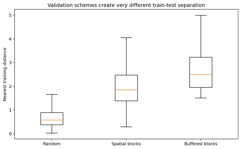
A simple distance diagnostic

For each test observation $j$, calculate

$$ d_j = \min_{i\in\mathcal T} d(s_j,s_i). $$

Then summarize:

• median nearest-training distance;
• 90th percentile;
• maximum distance.

A validation design is more representative of transfer when these distances resemble those expected at deployment.

Numerical distance example

Suppose five test locations have nearest-training distances $0.2,\ 0.3,\ 0.4,\ 0.5,\ 0.6$ km under random CV. The mean distance is

$$ \frac{0.2+0.3+0.4+0.5+0.6}{5} = \frac{2.0}{5} = 0.4\text{ km}. $$

Under blocked CV, suppose the distances are $2.1,\ 2.5,\ 2.7,\ 3.0,\ 3.2$. The mean is

$$ \frac{13.5}{5} = 2.7\text{ km}. $$

These two schemes evaluate very different levels of spatial separation. Nearest distance is a useful first diagnostic, not a complete description of information. A target with one nearby noisy observation and no others can be harder than one with several moderately close, precise observations. For anisotropic or network processes, measure distance in the geometry the model uses and consider directional coverage as well. Compare the distribution of these summaries with the intended deployment locations.

Spatial blocks

A common approach is to partition the study area into geographic blocks and hold out one or more complete blocks. For example, divide a rectangular region into:

• vertical strips;
• horizontal strips;
• square tiles;
• ecological regions;
• watersheds;
• administrative regions.

The blocks should reflect the intended deployment question.

Leave-one-block-out validation

Suppose the region is divided into five spatial blocks. For fold $k$:

1. block $k$ is the test set;
2. all other blocks are training data;
3. fit the entire modeling pipeline on training data;
4. predict the held-out block;
5. calculate performance.

Repeat for all five blocks. This creates five geographically distinct validation tasks.

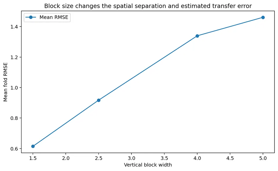
Block size matters

Very small spatial blocks can leave test observations almost adjacent to training observations. This weakens the intended geographic separation. Very large blocks create a harder transfer task but may leave too little training data. The block size should reflect:

• the spatial dependence range;
• the expected deployment distance;
• the spatial support of predictions;
• practical sample-size constraints.

Relationship to correlation range

Suppose residual correlation becomes weak after approximately

$$ 5\text{ km}. $$

If validation blocks are only

$$ 500\text{ m} $$

wide, test observations near a block edge can still have strongly correlated training observations immediately outside the block. The validation task remains close to interpolation. Using blocks several kilometers wide may better assess geographic transfer. There is no universal rule such as:

block size must equal exactly one variogram range.

The dependence range is one useful input, not an automatic choice.

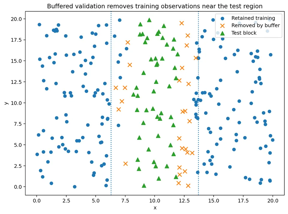
Buffered validation

A buffered split adds another layer of geographic separation. After selecting a test region, remove training observations within distance $b$ of the test region. The parameter $b$ is the buffer width.

What the buffer is doing

Suppose a held-out test block is surrounded by training observations immediately outside its boundary. Even when the test block itself is excluded, the task can remain easy. A buffer imposes an explicit minimum separation. If

$$ b=3\text{ km}, $$

training observations within 3 km of the test block are removed for that fold. This asks:

How well can the model predict when nearby training information is unavailable?

Numerical buffer example

Suppose a test site has a training observation

$$ 0.4\text{ km} $$

away. With no buffer, that observation remains available. With

$$ b=1\text{ km}, $$

it is removed. Suppose the next nearest training observation is

$$ 2.3\text{ km} $$

away. The effective test-to-training separation changes from $0.4$ to

$$ 2.3\text{ km}. $$

The validation task becomes substantially more difficult.

Buffers reduce training data

A larger buffer generally increases train-test separation but decreases the training sample size. This creates a tradeoff between separation and available training data. A very large buffer can produce unrealistic training sets with:

• too few observations;
• poor geographic coverage;
• missing predictor ranges.

Buffer width should therefore reflect deployment conditions rather than being maximized mechanically. When error rises with buffer width, part of the rise can come from greater separation and part from losing training observations or predictor coverage. Record retained training size and covariate support for each fold. A comparison that also subsamples unbuffered training data to a similar size can help distinguish these mechanisms, although it still does not make the geographic tasks identical.

Constructing a Buffer on an Explicit Set of Sites

Suppose sites lie at integer coordinates 0 through 10 along a line. Hold out sites 4, 5, and 6 as a test region. Without a buffer, the training coordinates are $0,1,2,3,7,8,9,10$. The three targets are one, two, and one unit from their nearest training sites, respectively.

Now remove every training site whose distance to any test site is at most two. This removes 2 and 3 on the left, and 7 and 8 on the right, leaving training sites $0,1,9,10$. Target distances become three, four, and three.

The buffer changes both spatial information and training size. A worse score can reflect either or both. Reporting only “two-unit buffer” conceals the actual prediction distances and how much training data remain. Also state the boundary convention: removing points at distance less than two would retain sites 2 and 8, producing another design.

For a two-dimensional polygon, distance to the test region means the minimum distance to that region, rather than distance to its centroid. A large polygon can have training sites far from its centroid but immediately adjacent to its boundary. If the target is an area average, exclusion should also respect overlapping measurement supports; two values with different centroids can share some of the same underlying observations.

Comparing performance with RMSE

A common prediction metric is root mean squared error:

$$ \boxed{ \mathrm{RMSE} = \sqrt{ \frac1m \sum_{j=1}^m (y_j-\hat y_j)^2 } }. $$

Smaller RMSE indicates better predictive accuracy on the response scale.

Worked RMSE example

Suppose four test observations are

$$ y= \begin{bmatrix} 10\\ 12\\ 14\\ 16 \end{bmatrix} $$

and predictions are

$$ \hat y= \begin{bmatrix} 11\\ 11\\ 13\\ 18 \end{bmatrix}. $$

The errors are

$$ -1,\ 1,\ 1,\ -2. $$

Squared errors are $1,\ 1,\ 1,\ 4$. Their mean is

$$ \frac{7}{4} = 1.75. $$

Therefore

$$ \mathrm{RMSE} = \sqrt{1.75} $$

$$ \boxed{ \mathrm{RMSE}\approx1.323 }. $$

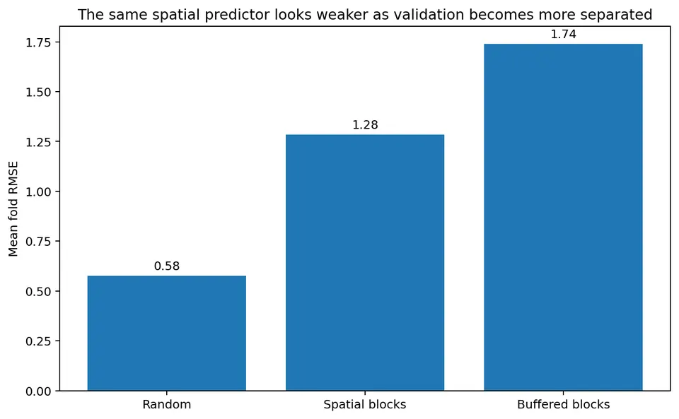
Validation design can change the RMSE substantially

A spatial predictor can achieve:

$$ \mathrm{RMSE}_{\text{random}} = 0.7, $$

$$ \mathrm{RMSE}_{\text{block}} = 1.8, $$

and

$$ \mathrm{RMSE}_{\text{buffered}} = 2.4. $$

These results are not contradictory. They describe different prediction tasks. The correct question is not:

Which RMSE is the true one?

It is:

Which validation geometry resembles deployment?

A toy spatial predictor

Inverse-distance weighting is used here only to demonstrate validation geometry. For a target $s_0$, the predictor is

$$ \hat y(s_0) = \frac{ \sum_{i\in\mathcal N_k(s_0)} w_i y_i }{ \sum_{i\in\mathcal N_k(s_0)}w_i }, $$

with

$$ w_i = \frac1{d(s_i,s_0)^p+\epsilon}. $$

Nearby training observations receive larger weight. This is intentionally simple. The purpose is not to recommend inverse-distance weighting as the preferred spatial model. Its purpose is simply to make the effect of train-test distance easy to see.

Why nearby training data make spatial prediction easier

Suppose a spatial process is smooth. Then

$$ y(s) \approx y(s+h) $$

for small $h$. If random CV leaves a training site very close to the test location, the model may recover much of the test value from local information. A blocked split reduces that advantage. This is why random CV often estimates interpolation skill rather than spatial transfer skill.

Leakage can be spatial

Validation can still be optimistic even when the split itself is geographically appropriate. Leakage occurs whenever information from held-out observations enters the training pipeline. Examples include:

• calculating neighborhood features using test observations;
• interpolating a covariate with the full dataset before splitting;
• estimating a variogram once using all observations;
• tuning bandwidth using held-out outcomes;
• normalizing variables using test data;
• imputing missing values using the complete dataset;
• defining a regional aggregate that includes the target observation.

Operations learned from the study's outcomes or training sample should be fitted within each fold when assessing the full procedure. A fixed external covariate map that will truly be available at deployment may legitimately be used at test sites. The issue is access to unavailable information, rather than whether a map covers both training and test regions. Document the source and timing of covariates and whether test outcomes influenced their construction.

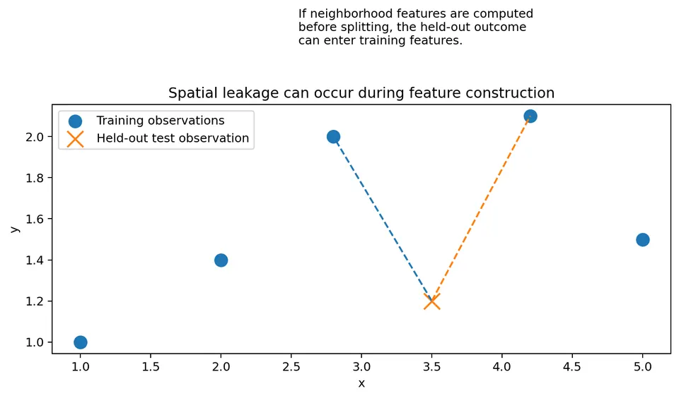
Leakage example: neighborhood mean

Suppose the feature for location $i$ is

$$ x_i^{\text{nbr}} = \frac1{k} \sum_{j\in N_k(i)}y_j. $$

This feature directly uses neighboring outcomes. If the neighborhood calculation is performed before splitting, a training row can contain information from a held-out test outcome. The model has then indirectly seen the held-out outcome. The correct procedure is:

1. split the data;
2. construct the neighborhood feature using training observations only;
3. fit the model;
4. calculate test features using only information that would be available at deployment.

Preprocessing must be fold-specific

The same principle applies to ordinary preprocessing. If a transformation is estimated from data, it belongs inside the resampling loop. Examples include:

• feature scaling;
• PCA;
• imputation;
• bandwidth selection;
• feature selection;
• spatial basis construction;
• variogram fitting;
• covariance-family selection.

This is ordinary machine-learning leakage with an added spatial dimension.

Cross-validation for kriging

Leave-one-out kriging removes one sampled site and predicts it from all remaining sites. This often leaves nearby observations in the training data. It therefore mainly assesses local interpolation. That may be exactly the right target for a densely sampled mapping problem. It is not necessarily appropriate for transfer to a new geographic region.

Kriging example

Suppose a monitoring site is omitted. Its two nearest remaining sites are only

$$ 150\text{ m} $$

and

$$ 220\text{ m} $$

away. Leave-one-out kriging can perform very well. But suppose the intended prediction area is

$$ 8\text{ km} $$

from the nearest monitor. Leave-one-out accuracy does not directly estimate performance under that deployment setting. A blocked or buffered holdout is more relevant.

Refit the variogram inside each fold

Suppose the workflow is:

1. estimate an empirical variogram;
2. select a covariance family;
3. fit covariance parameters;
4. krige;
5. evaluate test error.

If steps 1–3 use the full dataset, the held-out observations influence the model structure before prediction. That creates leakage. For a clean estimate of the full modeling procedure, fit the variogram and covariance parameters using only the training observations in each fold.

When full-data covariance fitting may still be useful

Sometimes the goal is not to estimate the full model-selection pipeline. For example, an analyst may want to compare prediction formulas conditional on a covariance model fixed externally from previous studies. Then keeping that covariance model fixed can be scientifically justified. The validation design should state clearly which components are fixed and which are re-estimated.

Hyperparameter tuning and nested spatial validation

Choose validation block and buffer geometry from the deployment question and scientific separation scale. These define the target of assessment and should not be optimized simply to obtain the best score. Model type and predictive hyperparameters can then be selected using an inner validation design consistent with that target. If the same folds are then used to report final performance, the estimate can be optimistic because those folds influenced model selection. A stronger design is:

1. inner spatial CV for model selection;
2. outer spatial CV or final geographic test set for evaluation.

This is the spatial analogue of nested validation.

Outcome-Based Spatial Features Must Respect the Prediction Task

An externally measured elevation map can be available at every future prediction site. A neighbor's observed response is different information. If that response would be available when predicting, it can legitimately inform an interpolation model. If the goal is transfer to an unmeasured region, such nearby outcomes may not exist.

A neighborhood response feature must therefore be rebuilt using the permitted observations in each fold. Training examples should not include their own responses through a regional aggregate or through a smoothing operation that includes them. Where feature construction itself estimates a response relationship, an appropriate inner or out-of-fold construction may be needed to prevent a training row's target from leaking into its predictors.

For a simultaneous spatial lag model, forming Wy from the entire observed response vector during validation directly exposes held-out responses. Predict the held-out outcomes using the fitted joint model and the information allowed by deployment instead. Substituting the true held-out outcomes into their neighbors' predictors evaluates a different, easier conditional task. This issue can occur even if the coefficient estimator itself is statistically appropriate.

Final geographic test region

If the dataset is large enough, reserve a final geographic region that is never used for:

• feature engineering;
• hyperparameter tuning;
• covariance-family selection;
• block-size tuning;
• model comparison.

Use it only for the final performance estimate. This design most closely approximates a future geographic deployment.

Unsupported extrapolation cannot be validated away

Suppose training temperature values lie between $10^\circ C$ and $25^\circ C$. Deployment will occur in a region with temperatures $35^\circ C$ to $40^\circ C$. Random or blocked resampling of the original data cannot evaluate model behavior at 40°C because such conditions are absent. The data simply do not contain empirical evidence for that regime. This is a support problem, not a problem that can be solved by a more elaborate cross-validation scheme.

Covariate overlap

Spatial transfer should therefore assess not only geographic separation but also predictor overlap. For each test region, ask:

• Are predictor values represented in training?
• Are combinations of predictors represented?
• Is the land-cover or climate regime new?
• Are measurement systems comparable?

A geographically separated test set can still represent interpolation in covariate space. Conversely, a geographically nearby test site can still be extrapolative if its predictor values are novel.

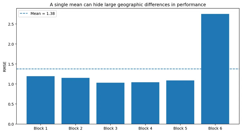
Fold-level performance matters

Suppose five spatial blocks have RMSE: $1.0,\ 1.1,\ 1.3,\ 2.8,\ 3.1$. The mean is

$$ \frac{1.0+1.1+1.3+2.8+3.1}{5} = 1.86. $$

Reporting only

$$ \text{mean RMSE}=1.86 $$

can hide substantial geographic heterogeneity. This is an unweighted mean of fold RMSEs, not a pooled observation-level RMSE. They generally differ even when folds have equal sizes, because taking a square root and averaging do not commute. Two regions are substantially harder than the others.

If fold $k$ has size $m_k$ and RMSE $r_k$, the pooled value is $\sqrt{\sum_km_kr_k^2/\sum_km_k}$. For equal fold sizes in this example, it is $\sqrt{(1^2+1.1^2+1.3^2+2.8^2+3.1^2)/5}\approx2.066$, rather than $1.86$. Equal-region averaging weights regions equally, while pooling weights observations equally. For deployment over geographic area or a target population, a further weighting scheme may be needed to represent that target.

Why spatial folds are not independent replicates

Adjacent or ecologically related blocks can share:

• climate;
• geology;
• measurement practices;
• unmeasured regional processes.

Five folds are therefore not equivalent to five independent experiments. A standard error calculated as though the folds were iid replicates can give a misleading sense of precision. Report:

• fold-level metrics;
• geographic maps;
• ranges or quantiles;
• the number and geometry of folds.

Mean performance versus deployment risk

Suppose average RMSE is acceptable but one important region performs very poorly. If deployment includes that region, the average alone may be insufficient. Validation should examine the distribution of errors across:

• geography;
• environmental conditions;
• distance from training;
• population groups or operational strata when relevant.

The reported metrics should support the actual decision. Uncertainty calibration is a separate part of that evaluation. If the model reports 90% prediction intervals, inspect held-out coverage, interval widths, and their variation by distance, region, and predictor novelty. Coverage alone can be made high by very wide intervals, while a low average RMSE can coexist with overconfident uncertainty in a sparsely sampled region. Use an observation-prediction interval for held-out noisy measurements and distinguish it from a latent-field interval.

Weighting Regions and Weighting Observations Give Different Scores

Suppose region A has 100 test observations with RMSE one, while B has 10 test observations with RMSE three. Their squared-error sums are 100 and 90. Pooling observations gives

$$ \mathrm{RMSE}_{\mathrm{pooled}} =\sqrt{\frac{100+90}{100+10}} \approx1.3143. $$

The mean of region RMSEs is $(1+3)/2=2$. Giving the two regions equal weight in mean squared error, then taking the square root, gives $\sqrt{(1+9)/2}\approx2.2361$. These differences arise from two choices: which units receive equal weight and whether the square root is taken before or after averaging.

If deployment selects a person from a population concentrated in A, an observation- or population-weighted loss may be relevant. If it selects one new region with equal probability and the cost is squared prediction error within that region, equal-region MSE is relevant. Neither should be substituted for the other because it produces a more favorable number. State the target weighting before comparing models, and use identical held-out observations and weights for each comparison.

Uncertainty in Average Loss Includes Spatial Covariance

For held-out losses $L_1,\ldots,L_m$, the average has variance

$$ \mathrm{Var}(\bar L) =\frac1{m^2}\left[\sum_i\mathrm{Var}(L_i) +2\sum_{i<j}\mathrm{Cov}(L_i,L_j)\right]. $$

Nearby prediction errors can make those loss covariances nonzero. Under the illustrative assumption of equal loss variance and common pairwise correlation $\rho_L$, the variance is multiplied by $1+(m-1)\rho_L$ relative to an independence calculation. With 20 losses and $\rho_L=0.2$, that multiplier is 4.8, giving an equivalent independent-loss count of about 4.17 for this average.

This does not supply a universal correction for real spatial data: correlations depend on geometry, loss, fitted model, and sampling design. It explains why many nearby test points cannot simply be counted as independent evidence about performance. Cross-validation folds add another dependence through overlapping training sets. Region-based resampling or model-based uncertainty calculations require enough appropriate units and a clear choice about whether the fitted model is fixed or refitted in each replicate.

For model comparisons, paired loss differences on the same held-out units often provide the relevant target, rather than two unrelated standard errors for two mean scores. Their spatial dependence still needs to be represented. Repeating arbitrary block origins measures sensitivity to split construction; it does not create new independent landscapes.

Block orientation can matter

Suppose a process changes mainly east-to-west. Vertical holdout strips may create stronger extrapolation than horizontal strips. If transport follows a river or prevailing wind, directional blocking may be scientifically meaningful. Spatial validation geometry should follow the expected deployment mechanism whenever possible.

Leave-region-out validation

Natural regions can sometimes provide more meaningful folds than arbitrary geometric blocks. Examples include:

• watersheds;
• hospitals;
• cities;
• farms;
• ecological reserves;
• administrative districts.

Leave-one-region-out validation asks:

Can the model transfer to a genuinely new region of the same type?

This is often easier to interpret scientifically than arbitrary geometric blocking.

Repeated spatial validation

A single blocking scheme can be sensitive to arbitrary boundary placement. One response is to repeat spatial blocking with different:

• origins;
• orientations;
• region selections.

This reveals how sensitive the results are to validation geometry. However, repeated folds are still not independent experiments. The purpose is robustness analysis, not artificial inflation of the effective sample size.

Buffer width as a sensitivity parameter

Instead of choosing a single buffer width, compare several plausible values:

$$ b=0,\ 1,\ 2,\ 4\text{ km}. $$

If performance degrades sharply as $b$ increases, the model relies strongly on very local training information. This can be scientifically informative. It answers:

How quickly does predictive skill decay as we remove nearby observations?

Block-size sensitivity as a diagnostic

Similarly, evaluate several block sizes. Small blocks may approximate interpolation. Larger blocks approximate increasingly difficult transfer. The resulting curve is not merely a tuning exercise. It shows how prediction performance changes as spatial separation increases. This can be more informative than a single cross-validation score.

Comparing validation schemes

A useful report might include:

These designs answer different questions. Do not rank them by difficulty and assume that the hardest design is automatically the most appropriate.

A complete spatial-validation workflow

Define deployment

Write down:

• where predictions will be made;
• expected distance to training data;
• whether new regions are expected;
• whether predictor conditions may be novel.

Map the data

Inspect:

• sampling density;
• clusters;
• gaps;
• boundaries;
• regional differences.

Estimate dependence scale

Use:

• residual variograms;
• Moran diagnostics;
• domain knowledge.

This helps inform block and buffer sizes.

Choose validation geometry

Select:

• random;
• blocked;
• buffered;
• leave-region-out;
• multiple schemes.

Put all preprocessing inside folds

Prevent both spatial and ordinary leakage.

Refit model components inside folds

When estimating the full modeling procedure, refit:

• feature engineering;
• covariance parameters;
• hyperparameters.

Record train-test separation

Summarize nearest-training distances.

Report fold-level metrics

Do not report only the overall mean performance.

Inspect covariate support

Check whether held-out conditions are represented in training.

Reserve final geographic testing if possible

Keep model selection separate from final evaluation.

Common mistakes

Using random CV for a regional-transfer claim

Random CV usually leaves nearby training observations available.

Choosing blocks that are too small

Test observations can remain almost adjacent to training data.

Choosing a huge buffer without considering deployment

A buffer should mimic the real information gap rather than maximize difficulty.

Computing spatial features before splitting

This can leak held-out information into training.

Fitting a variogram once on the full dataset during CV

The test fold influences covariance estimation.

Reporting only mean RMSE across spatial folds

Regional variation may be large.

Treating folds as independent experimental replicates

Spatial folds often share broad processes.

Assuming blocked CV solves extrapolation

It does not create evidence for predictor conditions absent from the dataset.

Tuning and evaluating on the same spatial folds

Model selection can make reported performance optimistic.

Compact worked comparison

Suppose a spatial model is evaluated three ways.

Random CV

Median test-to-training distance:

$$ 0.3\text{ km}. $$

RMSE: $0.8$.

Blocked CV

Median distance:

$$ 2.5\text{ km}. $$

RMSE: $1.6$.

Buffered blocked CV

Median distance:

$$ 4.2\text{ km}. $$

RMSE: $2.1$. A useful interpretation is:

Predictive error increases as nearby training information is removed. The random-CV result describes local interpolation, while the buffered result is more representative of prediction several kilometers from sampled sites.

A poor interpretation is:

Buffered CV proves the model is bad.

The model may perform very well for interpolation but poorly for transfer.

Worked Comparison: A Local Predictor and a Trend Model

Consider these observed values along the eleven-site line:

Hold out coordinates 4, 5, and 6. Compare two prespecified prediction rules: use the nearest training response, averaging equally when there is a distance tie; or fit an ordinary least-squares line to training response versus coordinate. Evaluate each rule using the same targets with and without the two-unit buffer defined above.

Without the buffer, nearest-site predictions are 11.9, 12.5, and 13.1. The middle target is equally distant from sites 3 and 7, so its prediction is $(11.9+13.1)/2$. Against observed targets 11.8, 11.8, and 12.2, the RMSE is

$$ \sqrt{\frac{0.1^2+0.7^2+0.9^2}{3}}\approx0.6608. $$

With the buffer, nearest-site predictions become 11.1, 13.15, and 15.2, using sites 1 and 9. Their RMSE is approximately 1.9419. Nearby information was especially useful for tracking the locally flatter response around the held-out sites.

The fitted trend lines are approximately $10.35694+0.51111s$ without the buffer and $10.25122+0.55976s$ with it. Substituting the three test coordinates gives the following comparison:

The local rule performs better for the first information setting, while the trend model performs better for the second. These are calculated results for this small constructed dataset, not claims that either rule usually wins. The buffer also reduces training size, so the score change is not attributable to distance alone.

The example shows why a model can be useful for interpolation yet compare differently when local observations are unavailable. It also shows why one cannot select the validation geometry by whichever score favors a preferred model. Fix the deployment target and assessment design first; use separate development or inner validation for selection; then assess the selected procedure on appropriate held-out information. Three test values are enough to illustrate the calculation, but not to estimate a reliable regional-transfer risk or its uncertainty.

Questions students should be able to answer

1. Why can random cross-validation be optimistic for spatial prediction?
2. What is the difference between interpolation and spatial transfer?
3. Why can no resampling design validate unsupported extrapolation?
4. What does nearest train-to-test distance tell us?
5. Why does block size matter?
6. What does a buffer accomplish?
7. Why can a larger buffer increase RMSE?
8. Why should preprocessing occur inside each fold?
9. Why can a neighborhood feature leak test information?
10. Why should a variogram sometimes be re-estimated inside each training fold?
11. Why are five spatial folds not equivalent to five independent experiments?
12. Why should fold-level metrics be reported?
13. What is the purpose of a final geographic test region?
14. Why can block orientation matter?
15. When is leave-region-out validation more interpretable than square blocks?