Correlation
Correlation is a statistical measure that quantifies the strength and direction of the linear relationship between two variables. It is a fundamental concept in statistics, enabling researchers and analysts to understand how one variable may predict or relate to another. The most commonly used correlation coefficients are the Pearson correlation coefficient and the Spearman rank correlation coefficient.
Understanding Correlation
- A positive correlation occurs when, as one variable increases, the other tends to rise as well.
- A negative correlation means larger values of one variable tend to be paired with smaller values of the other. This describes association; it does not state that changing one causes the other to decrease.
- Lastly, a zero correlation indicates that there is no linear relationship between the variables.
Important Note: Correlation does not imply causation. A high correlation between two variables does not mean that one variable causes changes in the other.
Pearson Correlation Coefficient ($r$)
The Pearson correlation coefficient measures linear association between numerical variables. The variables need not be continuous or normally distributed for the coefficient to be computed. Positive sample variances are required, and finite positive population variances are required for the corresponding population quantity. Outliers can strongly influence the result because covariance uses products of deviations. Distributional and sampling assumptions enter when calculating uncertainty or tests, rather than the arithmetic definition.
Definition
The Pearson correlation coefficient $r$ is defined as:
$$ r = \frac{\text{Cov}(X, Y)}{\sigma_X \sigma_Y} $$
Where:
- $\text{Cov}(X, Y)$ is the covariance between variables $X$ and $Y$.
- $\sigma_X$ and $\sigma_Y$ are the standard deviations of $X$ and $Y$, respectively.
The same formula is used for the population correlation (with population moments) and for the sample correlation (with sample moments; the factors $1/(n-1)$ cancel between numerator and denominator).
Alternative Formula:
$$ r = \frac{\sum_{i=1}^{n} (X_i - \bar{X})(Y_i - \bar{Y})}{\sqrt{\sum_{i=1}^{n} (X_i - \bar{X})^2} \sqrt{\sum_{i=1}^{n} (Y_i - \bar{Y})^2}} $$
Where:
- $n$ is the number of observations.
- $X_i$ and $Y_i$ are the $i$-th observations of $X$ and $Y$.
- $\bar{X}$ and $\bar{Y}$ are the sample means of $X$ and $Y$.
Interpretation
- $r = 1$: Perfect positive linear correlation (all points on a line with positive slope).
- $r = -1$: Perfect negative linear correlation.
- $r = 0$: No linear correlation.
General Guidelines:
| Correlation Strength | Range (r) |
|---|---|
| Strong Positive Correlation | 0.7 ≤ r ≤ 1.0 |
| Moderate Positive Correlation | 0.3 ≤ r < 0.7 |
| Weak Positive Correlation | 0 < r < 0.3 |
| No Correlation | r = 0 |
| Weak Negative Correlation | -0.3 < r < 0 |
| Moderate Negative Correlation | -0.7 < r ≤ -0.3 |
| Strong Negative Correlation | -1.0 ≤ r ≤ -0.7 |
These cut-offs are conventional rules of thumb, not universal; what counts as "strong" depends on the field.
The coefficient is dimensionless because rescaling either measurement multiplies its covariance and standard deviation by matching factors. Positive unit conversions leave correlation unchanged; reversing the direction of one scale changes its sign. A correlation of $0.75$ is not a statement that 75% of observations follow a pattern. In simple least-squares regression with an intercept, its square, $0.5625$, equals the in-sample fraction of centered response variation explained by the fitted line. This interpretation has specific modeling and fitting conditions.
Example: Calculating Pearson's $r$
Dataset
Consider the following data on the number of hours studied ($X$) and test scores ($Y$):
| Observation ($i$) | Hours Studied ($X_i$) | Test Score ($Y_i$) |
|---|---|---|
| 1 | 1 | 50 |
| 2 | 2 | 60 |
| 3 | 3 | 70 |
| 4 | 4 | 80 |
| 5 | 5 | 90 |
Step 1: Calculate the Means
$$ \bar{X} = \frac{1}{5}(1 + 2 + 3 + 4 + 5) = \frac{15}{5} = 3 $$
$$ \bar{Y} = \frac{1}{5}(50 + 60 + 70 + 80 + 90) = \frac{350}{5} = 70 $$
Step 2: Calculate Deviations and Products
Compute $(X_i - \bar{X})$, $(Y_i - \bar{Y})$, and their products:
| $i$ | $X_i$ | $Y_i$ | $X_i - \bar{X}$ | $Y_i - \bar{Y}$ | $(X_i - \bar{X})(Y_i - \bar{Y})$ | $(X_i - \bar{X})^2$ | $(Y_i - \bar{Y})^2$ |
|---|---|---|---|---|---|---|---|
| 1 | 1 | 50 | -2 | -20 | 40 | 4 | 400 |
| 2 | 2 | 60 | -1 | -10 | 10 | 1 | 100 |
| 3 | 3 | 70 | 0 | 0 | 0 | 0 | 0 |
| 4 | 4 | 80 | 1 | 10 | 10 | 1 | 100 |
| 5 | 5 | 90 | 2 | 20 | 40 | 4 | 400 |
| Sum | 100 | 10 | 1000 |
Step 3: Compute the Pearson Correlation Coefficient
$$ r = \frac{\sum_{i=1}^{5} (X_i - \bar{X})(Y_i - \bar{Y})}{\sqrt{\sum_{i=1}^{5} (X_i - \bar{X})^2} \sqrt{\sum_{i=1}^{5} (Y_i - \bar{Y})^2}} = \frac{100}{\sqrt{10} \times \sqrt{1000}} $$
Compute the denominators:
$$ \sqrt{10} \approx 3.1623, \quad \sqrt{1000} \approx 31.6228 $$
Compute $r$:
$$ r = \frac{100}{3.1623 \times 31.6228} = \frac{100}{100} = 1 $$
Visualization
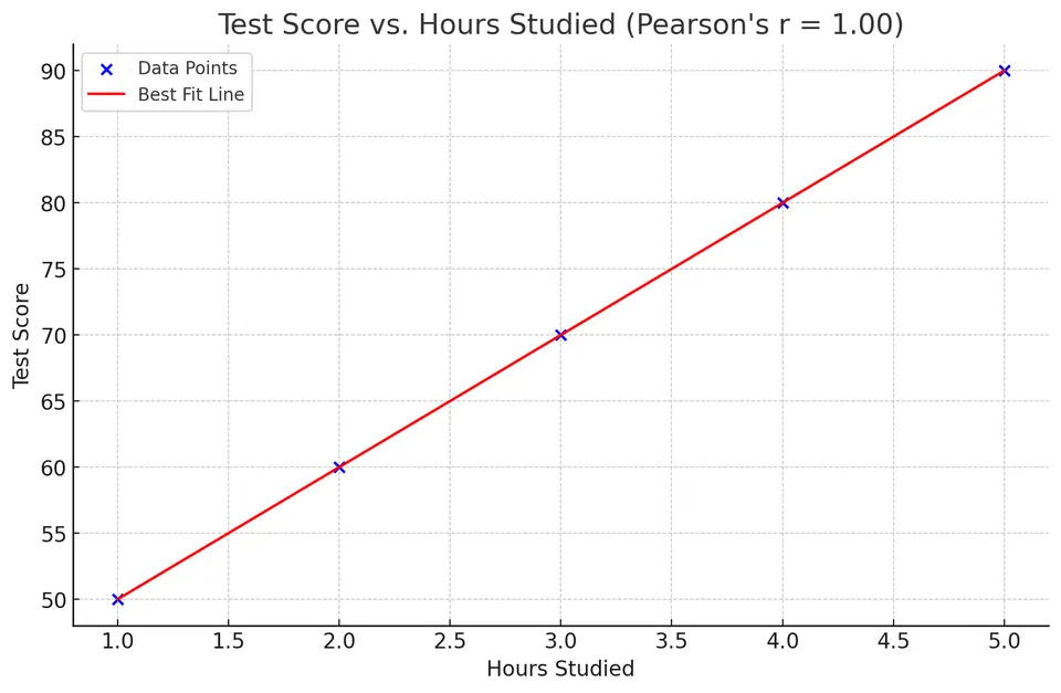
Pearson's $r = 1$ indicates a perfect positive linear relationship between hours studied and test scores. As the number of hours studied increases, the test score increases proportionally.
Spearman Rank Correlation Coefficient ($r_s$)
The Spearman rank correlation coefficient measures the strength and direction of the monotonic relationship between two variables. It is the Pearson correlation computed on the ranks of the data. It is a non-parametric measure, meaning it does not assume a specific distribution for the variables and is less sensitive to outliers.
Definition
The Spearman correlation coefficient $r_s$ is defined as:
$$ r_s = 1 - \frac{6 \sum_{i=1}^{n} d_i^2}{n(n^2 - 1)} $$
Where:
- $d_i = R(X_i) - R(Y_i)$ is the difference between the ranks of $X_i$ and $Y_i$.
- $R(X_i)$ and $R(Y_i)$ are the ranks of $X_i$ and $Y_i$, respectively.
- $n$ is the number of observations.
This shortcut formula is exact only when there are no ties. With ties, assign average ranks and compute the Pearson correlation of the ranks instead.
For example, values $[10,10,30]$ receive ranks $[1.5,1.5,3]$, because the tied observations share the average of positions one and two. Ranking discards the size of a jump from 10 to 30 but preserves ordering. This makes Spearman correlation less sensitive to how extreme a value is, while leaving it sensitive to changes in rank, ties, dependence between observations, and the chosen sample.
Calculation Steps
- Assign Ranks to the data points in $X$ and $Y$ separately.
- Compute the Differences of Ranks $d_i$.
- Square the Differences $d_i^2$.
- Compute $r_s$ using the formula.
Example: Calculating Spearman's $r_s$
Using the same dataset:
| Observation ($i$) | Hours Studied ($X_i$) | Test Score ($Y_i$) |
|---|---|---|
| 1 | 1 | 50 |
| 2 | 2 | 60 |
| 3 | 3 | 70 |
| 4 | 4 | 80 |
| 5 | 5 | 90 |
Step 1: Assign Ranks
Since the data is already ordered, the ranks correspond to the order of observations.
| $i$ | $X_i$ | Rank $R(X_i)$ | $Y_i$ | Rank $R(Y_i)$ |
|---|---|---|---|---|
| 1 | 1 | 1 | 50 | 1 |
| 2 | 2 | 2 | 60 | 2 |
| 3 | 3 | 3 | 70 | 3 |
| 4 | 4 | 4 | 80 | 4 |
| 5 | 5 | 5 | 90 | 5 |
Step 2: Compute Differences of Ranks
Calculate $d_i = R(X_i) - R(Y_i)$:
| $i$ | Rank $R(X_i)$ | Rank $R(Y_i)$ | $d_i$ | $d_i^2$ |
|---|---|---|---|---|
| 1 | 1 | 1 | 0 | 0 |
| 2 | 2 | 2 | 0 | 0 |
| 3 | 3 | 3 | 0 | 0 |
| 4 | 4 | 4 | 0 | 0 |
| 5 | 5 | 5 | 0 | 0 |
| Sum | 0 |
Step 3: Compute Spearman's $r_s$
$$ r_s = 1 - \frac{6 \times 0}{5(5^2 - 1)} = 1 - 0 = 1 $$
Interpretation
Spearman's $r_s = 1$ indicates a perfect positive monotonic relationship between hours studied and test scores.
When to Use Spearman's $r_s$
- When data is ordinal.
- When the relationship between variables is monotonic but not necessarily linear.
- When there are outliers that might affect Pearson's $r$.
- When the scientific question concerns order or a monotonic relation. Non-normal marginals alone do not require replacing Pearson correlation; choose the summary according to the relationship of interest.
Comparison of Pearson's $r$ and Spearman's $r_s$
- Pearson's $r$ measures the strength of a linear relationship.
- Spearman's $r_s$ measures the strength of a monotonic relationship.
- Both coefficients range from -1 to 1.
- With no ties, $r_s=\pm1$ when the observations have exactly matching or reversed rank order, including a strictly monotonic nonlinear relation. With ties, use average ranks; equality requires the centered rank vectors to be proportional. A flat segment that introduces ties in only one variable can prevent perfect rank correlation. Pearson's $r=\pm1$ instead requires an exact affine relationship between the original nonconstant values.
- Spearman's $r_s$ is less sensitive to outliers and does not require the assumption of normality.
Correlation of Two Random Variables
For two random variables $X$ and $Y$ with positive variances, the population correlation coefficient $\rho_{XY}$ is defined as:
$$ \rho_{XY} = \frac{\text{Cov}(X, Y)}{\sigma_X \sigma_Y} $$
Where:
- $\text{Cov}(X, Y)$ is the covariance between $X$ and $Y$.
- $\sigma_X$ and $\sigma_Y$ are the standard deviations of $X$ and $Y$.
Properties
| Property | Description |
|---|---|
| Range | $-1 \leq \rho_{XY} \leq 1$ |
| Symmetry | $\rho_{XY} = \rho_{YX}$ |
| Dimensionless | The correlation coefficient is unitless. |
| Linearity | If $\rho_{XY} = \pm 1$, then $Y=a+bX$ with probability 1 (and $b$ has the sign of $\rho_{XY}$). |
| Independence | Independence implies zero correlation when finite positive variances exist. The converse fails in general; for a jointly normal pair, zero correlation is sufficient for independence. |
Interpretation
- $\rho_{XY} > 0$: Positive linear relationship.
- $\rho_{XY} < 0$: Negative linear relationship.
- $\rho_{XY} = 0$: No linear relationship.
Example with Random Variables
Suppose $X$ and $Y$ are random variables with the following properties:
- $\mu_X = \mathbb{E}[X] = 5$
- $\mu_Y = \mathbb{E}[Y] = 10$
- $\sigma_X = \sqrt{\text{Var}(X)} = 2$
- $\sigma_Y = \sqrt{\text{Var}(Y)} = 4$
- $\text{Cov}(X, Y) = 6$
Compute the correlation coefficient:
$$ \rho_{XY} = \frac{\text{Cov}(X, Y)}{\sigma_X \sigma_Y} = \frac{6}{2 \times 4} = \frac{6}{8} = 0.75 $$
Interpretation:
- A correlation coefficient of $0.75$ indicates a strong positive linear relationship between $X$ and $Y$ by the conventional guidelines above.
- The covariance is consistent with the bound $|\text{Cov}(X,Y)|\le\sigma_X\sigma_Y=8$.
Important Considerations
Correlation vs. Causation
- Correlation does not imply causation. A high correlation between two variables does not mean that one variable causes changes in the other.
- A confounding variable (or lurking variable) may influence both correlated variables, creating a statistical association without a direct causal link. For example, ice cream sales and drowning incidents are positively correlated, but neither causes the other — the confounding variable is hot weather, which independently increases both.
- Spurious correlations can arise purely by chance, especially when testing many variable pairs simultaneously or when working with small sample sizes. Always consider the underlying mechanism before drawing conclusions from observed correlations.
Outliers
- Pearson's $r$ is sensitive to outliers, which can distort the correlation coefficient.
- Spearman's $r_s$ is more robust to outliers due to ranking.
Non-linear Relationships
- Variables can have a strong non-linear relationship but a low Pearson correlation coefficient.
- If the relationship is monotonic (for example $Y=e^X$), Spearman's $r_s$ will detect it.
- If the relationship is non-monotonic (for example $Y=X^2$ with $X$ symmetric about zero), both coefficients can be near zero even though $Y$ is a function of $X$.
Assumptions of Pearson's $r$
- Linearity: the relationship between $X$ and $Y$ should be approximately straight, because $r$ measures only linear association.
- No extreme outliers or leverage points, which can dominate $r$.
- Independent bivariate normal observations give the exact usual t test for zero population correlation. The Fisher-z confidence interval is a large-sample approximation even under that model. Other inferential methods can be used under different assumptions; normality is not required to compute the descriptive coefficient.
- Constant spread (homoscedasticity) is not required for $r$ to be defined, but a funnel-shaped scatter means a single $r$ summarizes the relationship poorly.
If these conditions are violated, Pearson's $r$ may not be an appropriate summary, and a rank-based or other measure may be preferable.