Time Series Modeling
Time-series modeling is an iterative process of specifying structure, estimating parameters, diagnosing what remains unexplained, and testing forecasts on future-like data. Choosing an equation is only one step; transformations, initial conditions, residual behavior, and the forecast information set are part of the model as well.
A useful model is parsimonious enough to estimate reliably, flexible enough to capture the important dependence, and transparent enough to diagnose. Information criteria can narrow a candidate set, but residual checks and chronological forecast evaluation determine whether the selected model is actually adequate for its intended use.
Formula reference
| Topic / model | General formula | Use / special case |
|---|---|---|
| AR($p$) | $Y_t=c+\sum_{i=1}^{p}\phi_iY_{t-i}+\varepsilon_t$ | Lagged observations are observed regressors. |
| MA($q$) | $Y_t=\mu+\varepsilon_t+\sum_{j=1}^{q}\theta_j\varepsilon_{t-j}$ | Lagged innovations are latent. |
| ARMA($p,q$) | $\phi(B)(Y_t-\mu)=\theta(B)\varepsilon_t$ | Stationary short-memory linear model. |
| ARIMA($p,d,q$) | $\phi(B)(1-B)^dY_t=c+\theta(B)\varepsilon_t$ | Adds ordinary differencing. |
| SARIMA | $\Phi(B^s)\phi(B)(1-B^s)^D(1-B)^dY_t=\Theta(B^s)\theta(B)\varepsilon_t$ | Adds seasonal dynamics and differencing. |
| OLS for AR design | $\hat\beta=(X^\top X)^{-1}X^\top y$ | Requires full column rank; numerical solvers are preferred to explicit inversion. |
| Gaussian innovation log-likelihood | $\ell_t=-\tfrac12[\log(2\pi)+\log F_t+v_t^2/F_t]$ | State-space/innovations form; sum over $t$. |
| Residual | $\hat\varepsilon_t=y_t-\hat y_{t\mid t-1}$ | One-step unexplained component. |
| Residual ACF | $\hat\rho(h)=\frac{\sum_{t=h+1}^{T}(\hat\varepsilon_t-\bar\varepsilon)(\hat\varepsilon_{t-h}-\bar\varepsilon)}{\sum_{t=1}^{T}(\hat\varepsilon_t-\bar\varepsilon)^2}$ | Checks remaining linear dependence. |
| Ljung-Box | $Q(m)=T(T+2)\sum_{h=1}^{m}\hat\rho(h)^2/(T-h)$ | Joint residual-autocorrelation diagnostic. |
| AIC | $\mathrm{AIC}=-2\ell+2k$ | Lower is preferred within comparable likelihood fits. |
| AICc | $\mathrm{AICc}=\mathrm{AIC}+2k(k+1)/(n-k-1)$ | Small-sample correction to AIC. |
| BIC | $\mathrm{BIC}=-2\ell+k\log n$ | Penalizes complexity more strongly as $n$ grows. |
| AR stationarity/causality | $\phi(z)=0\Rightarrow\lvert z\rvert>1$ | Standard backshift-root condition. |
| MA invertibility | $\theta(z)=0\Rightarrow\lvert z\rvert>1$ | Selects the stable innovation representation. |
| Forecast error | $e_{t,h}=y_{t+h}-\hat y_{t+h\mid t}$ | Evaluate on chronological future-like origins. |
| MAE / RMSE | $\mathrm{MAE}=n^{-1}\sum\lvert e_i\rvert$, $\mathrm{RMSE}=\sqrt{n^{-1}\sum e_i^2}$ | Complement likelihood criteria with out-of-sample loss. |
Worked calculation: fit, complexity, and diagnostics
Suppose two likelihood-based candidates have the following summaries:
| Model | log-likelihood | number of parameters |
|---|---|---|
| A | $-100$ | 3 |
| B | $-96$ | 6 |
Using
$$ \mathrm{AIC}=-2\ell+2k, $$
their AIC values are
$$ \mathrm{AIC}_A=200+6=206, \qquad \mathrm{AIC}_B=192+12=204. $$
Model B wins this narrow in-sample comparison, but it should not be accepted automatically. If B leaves a residual lag-12 spike while A has approximately white-noise residuals, A may be the more useful forecasting model. Compare candidates on the same observations, inspect residuals, and use temporal backtesting before treating a small information-criterion difference as meaningful.
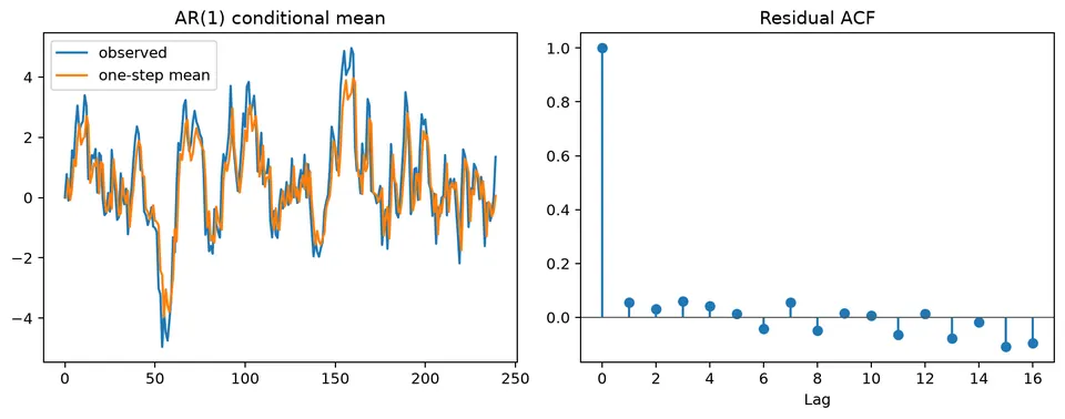
The figure shows the two parts of model assessment together: the fitted conditional mean should capture the systematic structure, and the residuals should no longer contain obvious predictable dependence.
Time-series modeling combines specification, parameter estimation, model selection, diagnostics, and forecast evaluation. The aim is not simply to minimize in-sample error, but to find a parsimonious model whose assumptions are reasonable, whose residuals contain little unexplained structure, and whose forecasts generalize to future observations.
Model Fitting
Different model classes require different estimation methods. In an autoregressive model, lagged observations are known and can be used as regressors. In MA and ARMA models, lagged innovations are unobserved, so estimation generally relies on likelihood, innovations recursions, or state-space methods.
The estimation method is part of the model specification. Initial conditions, treatment of missing values, and whether the likelihood is conditional or exact can affect numerical results in short samples.
Worked Example: Fitting an AR(2) Model
Consider
$$ Y_t=\beta_0+\beta_1Y_{t-1}+\beta_2Y_{t-2}+\varepsilon_t. $$
Use the short synthetic series
| $t$ | $Y_t$ |
|---|---|
| 1 | 1.0 |
| 2 | 2.0 |
| 3 | 1.5 |
| 4 | 3.0 |
| 5 | 2.5 |
| 6 | 4.0 |
Using observations $t=3,\dots,6$ gives
$$ \mathbf y= \begin{bmatrix} 1.5\\ 3.0\\ 2.5\\ 4.0 \end{bmatrix}, \qquad \mathbf X= \begin{bmatrix} 1&2.0&1.0\\ 1&1.5&2.0\\ 1&3.0&1.5\\ 1&2.5&3.0 \end{bmatrix}. $$
If $\mathbf X$ has full column rank, the least-squares estimator is
$$ \hat{\boldsymbol\beta} =(\mathbf X^\top\mathbf X)^{-1}\mathbf X^\top\mathbf y. $$
For this dataset,
$$ \mathbf X^\top\mathbf X = \begin{bmatrix} 4&9&7.5\\ 9&21.5&17\\ 7.5&17&16.25 \end{bmatrix}, $$
and
$$ \mathbf X^\top\mathbf y = \begin{bmatrix} 11\\ 25\\ 23.25 \end{bmatrix}. $$
Solving the normal equations gives approximately
$$ \hat\beta_0=0.328, \qquad \hat\beta_1=0.080, \qquad \hat\beta_2=1.195. $$
Thus the fitted conditional mean is
$$ \hat Y_t=0.328+0.080Y_{t-1}+1.195Y_{t-2}. $$
Here $\hat\beta_1+\hat\beta_2\approx1.275>1$ and both roots of $1-0.080z-1.195z^2$ have modulus below 1, so the fitted recursion is explosive: with only four equations and three parameters the fit is essentially interpolation. This example demonstrates only the mechanics of regression-style AR estimation. The fitted coefficients are not the end of the analysis: check the implied stability, residual dependence, competing orders, and out-of-sample performance before using the model.
Why the Design Matrix Needs Variation
If observations increase by a constant amount (for example $1,2,3,\ldots$), adjacent lag columns can become linearly dependent once an intercept is included. Then $\mathbf X^\top\mathbf X$ is singular, the inverse in the ordinary least-squares expression does not exist, and the coefficients are not uniquely identified.
This is a general lesson rather than a quirk of one example: inspect the design matrix and data variation before presenting or interpreting an inverse-based estimate.
Fitting MA and ARMA Models
An MA(2) model is
$$ Y_t=\mu+\varepsilon_t+\theta_1\varepsilon_{t-1}+\theta_2\varepsilon_{t-2}. $$
The lagged innovations are latent. Treating them as ordinary observed regressors is therefore not valid. Practical estimation commonly uses maximum likelihood, innovations algorithms, or state-space methods. Procedures such as Hannan-Rissanen can also provide useful starting estimates for ARMA likelihood optimization.
Comparison of Common Models
| Model | Main idea | Typical use | Important assumptions / cautions |
|---|---|---|---|
| AR($p$) | Current value depends on past values | Short-memory stationary dependence | Check stationarity and root location after any required transformation |
| MA($q$) | Current value depends on current and past innovations | Short-lived shock effects | Innovations are latent; invertibility matters for identification |
| ARMA($p,q$) | Combines AR and MA terms | Stationary linear series | Use parsimonious order selection and residual diagnostics |
| ARIMA($p,d,q$) | ARMA structure after differencing | Integrated or stochastic-trend series | Use the smallest justified differencing order |
| SARIMA | ARIMA plus seasonal AR, MA, and differencing terms | Regular seasonal structure | Seasonal period and seasonal differencing must match the data mechanism |
| SES / Holt / Holt-Winters / ETS | Recursive level, trend, and seasonal states | Forecasting evolving level/trend/seasonality | Different structures imply different error and state dynamics |
| VAR | Several variables depend on their joint lags | Multivariate linear dynamics | Lag order, stability, and cointegration matter; predictability is not automatically causal |
| ARCH/GARCH | Conditional variance evolves over time | Volatility clustering | Usually modeled after specifying an adequate conditional mean |
The table is a model map, not a ranking. The appropriate class depends on what is being forecast, which structures are present, and which assumptions remain plausible after diagnostics.
A Practical Identification and Validation Workflow
- Explore the series. Plot the data and identify trend, seasonality, missingness, outliers, structural breaks, and changing variance.
- Assess stationarity. Use plots, ACF behavior, and tests such as ADF/KPSS as supporting evidence.
- Transform when needed. Apply variance stabilization, detrending, ordinary differencing, or seasonal differencing only when justified.
- Propose candidate orders. Use ACF/PACF patterns and domain knowledge as heuristics rather than mechanical rules.
- Estimate parameters. Use a method appropriate to the model class.
- Compare parsimonious candidates. Use AIC, AICc, or BIC only among models fitted to comparable data and likelihoods.
- Diagnose residuals. Check residual time plots, ACF/PACF, squared residuals, and relevant tests such as Ljung-Box.
- Evaluate forecasts temporally. Preserve chronology with holdouts or rolling/expanding origins.
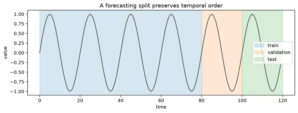
The figure emphasizes the final step: model selection is incomplete until the complete procedure is tested on future-like observations without information leakage.
ARMA Identification and Estimation Checklist
For a stationary series, a common ARMA workflow is:
- propose a small set of $p$ and $q$ values from ACF/PACF behavior and domain knowledge;
- decide whether a mean or intercept term is appropriate;
- estimate AR and MA coefficients with a suitable numerical method;
- estimate the innovation variance;
- compare candidates using diagnostics and information criteria;
- verify that residuals no longer contain material serial dependence.
For pure AR models, Yule-Walker or Burg estimators can be useful. Innovations algorithms target MA structure, while Hannan-Rissanen can provide starting values before likelihood optimization.
Order Selection with AICc
The corrected Akaike Information Criterion (AICc) adjusts AIC for finite samples. One common form is
$$ \mathrm{AICc} =\mathrm{AIC} +\frac{2k(k+1)}{n-k-1}, $$
where $k$ is the number of estimated parameters counted in the likelihood and $n$ is the effective sample size.
Lower values indicate a better fit-complexity tradeoff within a comparable candidate set. Parameter-count and effective-sample conventions vary across implementations, so check the software documentation when reproducing exact values.
Parameter Redundancy
An over-parameterized ARMA model can sometimes represent a simpler process if the AR and MA polynomials share common factors. Such cancellations make parameters redundant and can weaken identification.
Prefer reduced representations without common factors. If estimated roots nearly cancel, treat the apparent complexity with caution rather than interpreting each coefficient as a separate dynamic mechanism.
Model Selection Is Not Only About Fit
A more complex model can often reduce in-sample error, but that does not guarantee better forecasting. Prefer the simplest model that captures the important dependence, leaves reasonably well-behaved residuals, and performs competitively on future-like observations.
Connections to Other Notes
- See stationarity.md before interpreting AR/MA/ARIMA models.
- See autocorrelation_function.md for ACF/PACF-based identification.
- See autoregressive_models.md and moving_average_models.md for model-specific properties.
- See arima_models.md for differencing and seasonal ARIMA models.
- See randomness_tests.md for residual checks.
- See forecasting.md for forecast construction and uncertainty.
Student guide: an end-to-end modeling record
A time-series model is a set of assumptions about the conditional mean, temporal dependence, new shocks, variance behavior, and information available for prediction. Record these assumptions explicitly before comparing software summaries.
A table of coefficients alone does not tell a reader which observations were used, how missing values were handled, which transformations were applied, or whether the residuals are adequate.
Start with the target and the index
Record:
- the response variable and its units;
- the timestamp and sampling interval;
- whether timestamps are regular;
- the forecast horizon;
- the difference between observation time and release time;
- the deployment decision the forecast supports.
For example, a monthly sales forecast issued on the last day of March may use completed March sales, while a forecast issued on March 10 may have only partial March information. The timestamp is therefore part of the model's information set, not just a plotting label.
Explore before fitting
Inspect the level series, relevant transformations, first and seasonal differences, rolling mean and variance, missingness and outliers, ACF/PACF, known calendar effects, and possible structural breaks.
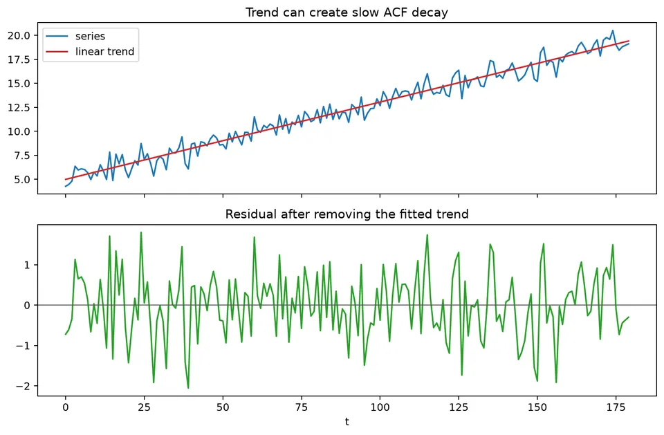
The detrending figure shows why preprocessing should follow the mechanism. Removing a deterministic trend can reveal stationary residual structure, while differencing answers a different question by modeling changes rather than deviations around a fitted trend.
An ACF that decays slowly may reflect a unit root, deterministic trend, seasonal pattern, or structural break. It is evidence to investigate, not a diagnosis by itself.
Estimation mechanics
For AR($p$), lagged observations are observed:
$$ y_t=c+\phi_1y_{t-1}+\cdots+\phi_py_{t-p}+\varepsilon_t. $$
For MA($q$), lagged innovations are not observed:
$$ y_t=\mu+\varepsilon_t+\theta_1\varepsilon_{t-1}+\cdots+\theta_q\varepsilon_{t-q}. $$
The innovations must be inferred recursively or through an equivalent state-space representation. Treating them as known regressors changes the estimation problem.
For a Gaussian state-space or innovations representation, log-likelihood contributions often have the form
$$ -\frac12\left[\log(2\pi)+\log(F_t)+\frac{v_t^2}{F_t}\right]. $$
Initial-state treatment can affect exact likelihood values in short samples, so compare candidate models under consistent conventions.
Numerical order selection
Suppose one model has $\ell=-100$ and $k=3$:
$$ \mathrm{AIC}=-2(-100)+2(3)=206. $$
A larger model has $\ell=-96$ and $k=6$:
$$ \mathrm{AIC}=-2(-96)+2(6)=204. $$
The larger model is preferred by AIC in this comparison, but the difference is not evidence by itself that forecasts improve. BIC applies a stronger sample-size-dependent penalty:
$$ \mathrm{BIC}=-2\ell+k\log n. $$
Use AICc when the effective sample is not large relative to the parameter count, and compare only models fitted to comparable observations and likelihood definitions.
Residuals as a model check
Let
$$ \hat\varepsilon_t=y_t-\hat y_{t|t-1} $$
be one-step residuals. A useful residual sequence should have approximately zero mean, little remaining serial correlation, reasonably stable variance, no unexplained trend or break, and no systematic relation to fitted values or predictors.
For residual autocorrelation,
$$ \hat\rho(h) =\frac{\sum_{t=h+1}^{T} (\hat\varepsilon_t-\bar\varepsilon) (\hat\varepsilon_{t-h}-\bar\varepsilon)} {\sum_{t=1}^{T}(\hat\varepsilon_t-\bar\varepsilon)^2}. $$
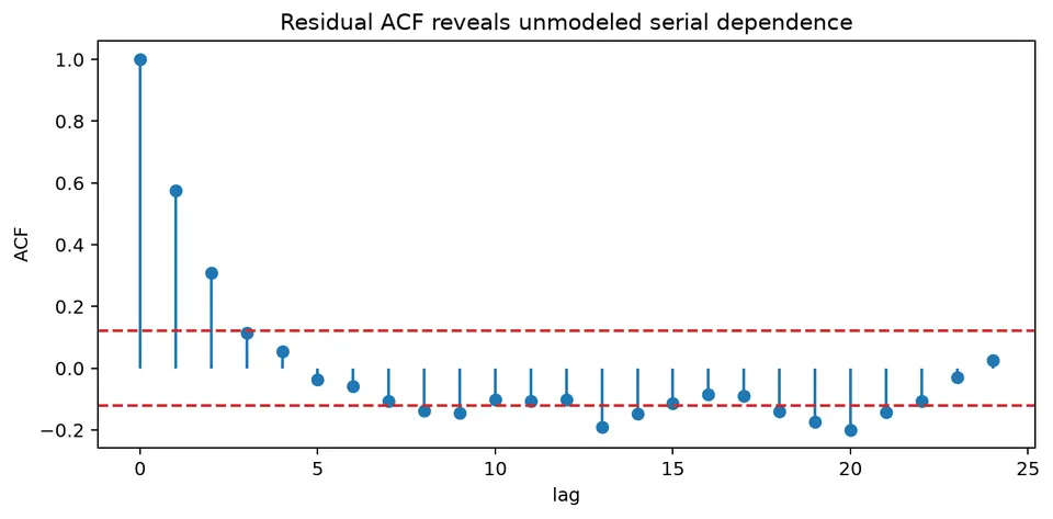
The residual ACF shows whether linear dependence remains after fitting. A visible spike suggests a missing dynamic term, seasonal feature, predictor, or structural component, but the plot alone does not tell which one.
The Ljung-Box statistic through lag $m$ is
$$ Q(m)=T(T+2)\sum_{h=1}^{m}\frac{\hat\rho(h)^2}{T-h}. $$
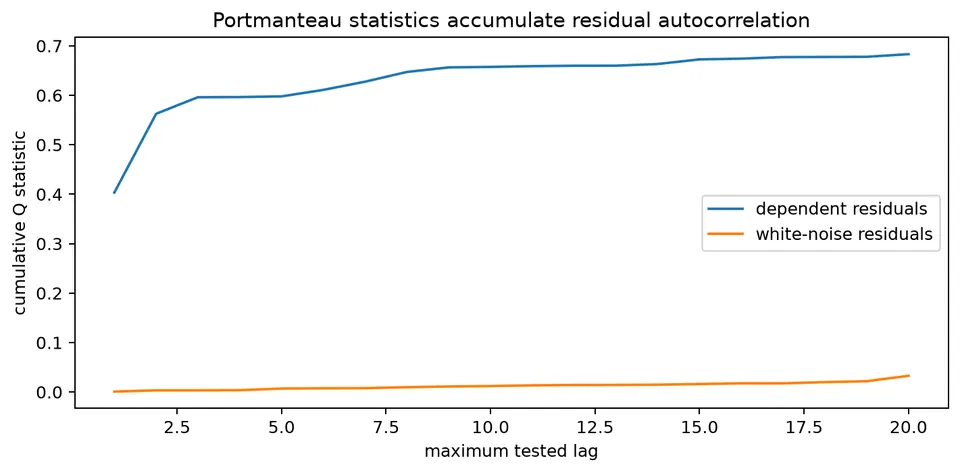
The figure reinforces that the test aggregates evidence across several lags. A small p-value says the residuals retain linear dependence at one or more tested lags; it does not prescribe the replacement model.
Residual variance and distribution
A residual ACF near zero does not establish independent, homoskedastic residuals. Inspect squared residuals and their dependence as well.
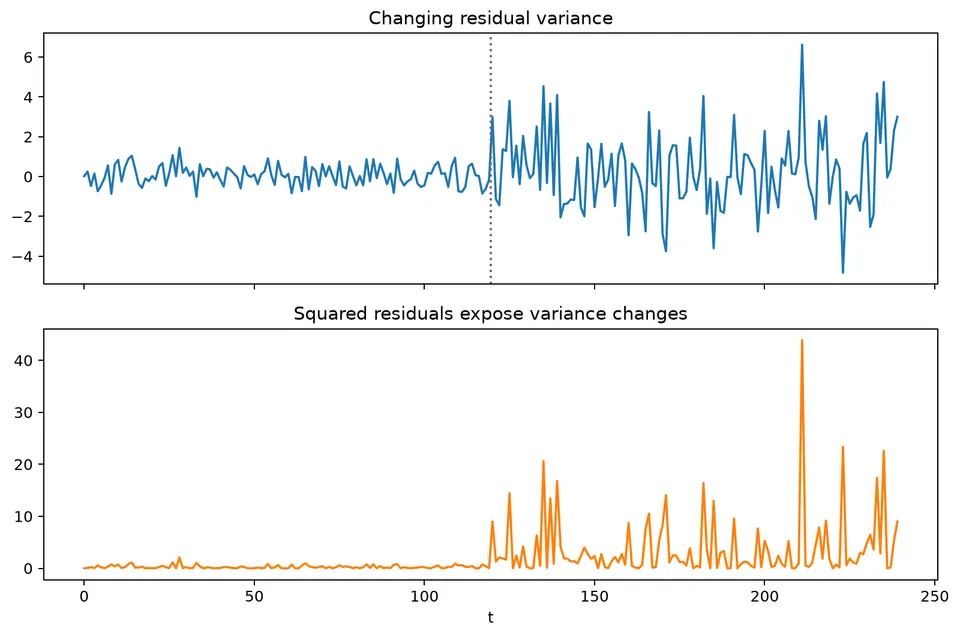
Changing residual spread indicates that the conditional variance may need separate modeling.
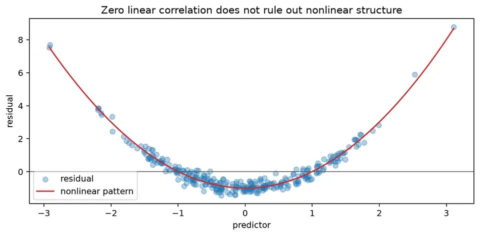
A residual plot can also reveal nonlinear patterns that a linear mean model cannot capture even when ordinary autocorrelation is small.
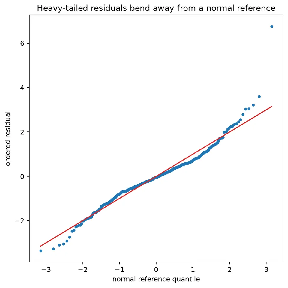
Heavy tails or skewness can make Gaussian prediction intervals poorly calibrated even when the conditional mean is adequate. The relevant distributional assumption should match the forecast objective, especially when tail probabilities matter.
Structural breaks
A single stable parameter set can average over multiple regimes. After a break, residuals may show a level shift, a change in persistence, a variance jump, or a change in seasonal amplitude.
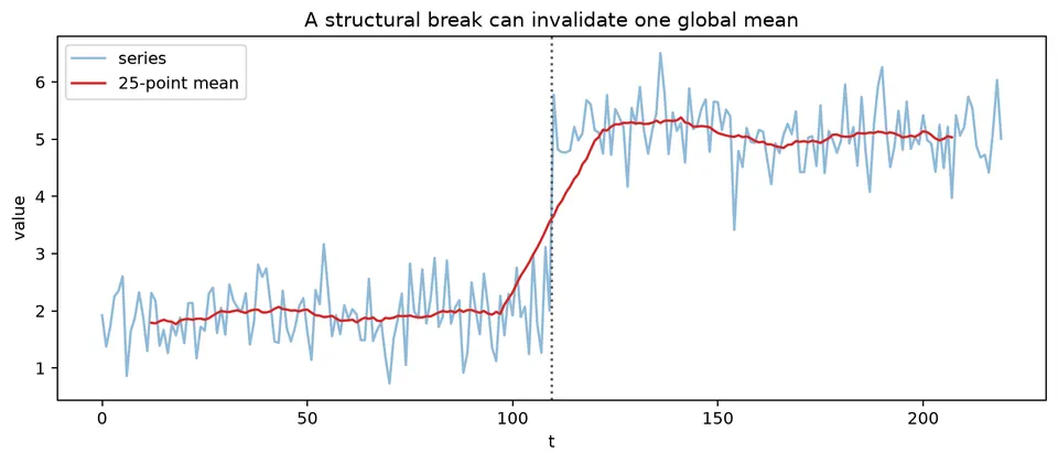
The break figure shows why an isolated global fit can be misleading: parameters that describe the pre-break period may no longer represent the post-break process.
Possible responses include a break indicator, separate regimes, rolling estimation, time-varying state-space parameters, or a documented model reset. Do not automatically discard unusual observations when the event itself may recur and matter for forecasting.
A model comparison table
Keep an auditable record:
| candidate | transformation | parameters | AIC | residual ACF | backtest MAE | notes |
|---|---|---|---|---|---|---|
| naive | none | 0 | — | — | baseline | |
| AR(1) | none | 2 | ||||
| ARIMA | first difference | |||||
| seasonal model | seasonal difference |
The chosen model should be the simplest candidate that captures the important structure and performs acceptably on future-like data. A lower in-sample criterion paired with poor residuals is a warning, not a victory.