Covariance
Covariance averages products of deviations from two means. When both deviations have the same sign, their product is positive; when their signs differ, it is negative. The average therefore indicates the direction of linear co-variation, while its numerical size also reflects the units and variability of both measurements:
- A positive covariance implies that as one variable increases, the other tends to increase as well.
- A negative covariance suggests that as one variable increases, the other tends to decrease.
- A zero covariance indicates no linear relationship between the variables.
Definition
The covariance between two random variables $X$ and $Y$ is defined as the expected value (mean) of the product of their deviations from their respective means:
$$ \text{Cov}(X, Y) = \mathbb{E}\left[ (X - \mu_X)(Y - \mu_Y) \right] $$
Where:
- $\text{Cov}(X, Y)$ is the covariance between $X$ and $Y$.
- $\mathbb{E}$ denotes the expected value operator.
- $\mu_X = \mathbb{E}[X]$ is the mean of $X$.
- $\mu_Y = \mathbb{E}[Y]$ is the mean of $Y$.
Alternative Expression
By expanding the definition and applying the linearity properties of expectation, covariance can also be expressed as:
$$ \text{Cov}(X, Y) = \mathbb{E}[XY] - \mathbb{E}[X] \mathbb{E}[Y] $$
Derivation:
- Start with the definition:
$$ \text{Cov}(X, Y) = \mathbb{E}\left[ (X - \mu_X)(Y - \mu_Y) \right] $$
- Expand the product inside the expectation:
$$ \text{Cov}(X, Y) = \mathbb{E}\left[ XY - X \mu_Y - \mu_X Y + \mu_X \mu_Y \right] $$
- Use the linearity of expectation:
$$ \text{Cov}(X, Y) = \mathbb{E}[XY] - \mu_Y \mathbb{E}[X] - \mu_X \mathbb{E}[Y] + \mu_X \mu_Y $$
- Recognize that $\mu_X = \mathbb{E}[X]$ and $\mu_Y = \mathbb{E}[Y]$:
$$ \text{Cov}(X, Y) = \mathbb{E}[XY] - \mu_Y \mu_X - \mu_X \mu_Y + \mu_X \mu_Y = \mathbb{E}[XY] - \mu_X \mu_Y $$
Thus, we arrive at:
$$ \text{Cov}(X, Y) = \mathbb{E}[XY] - \mathbb{E}[X] \mathbb{E}[Y] $$
Interpretation
- Positive Covariance ($\text{Cov}(X, Y) > 0$): Indicates that $X$ and $Y$ tend to increase or decrease together.
- Negative Covariance ($\text{Cov}(X, Y) < 0$): Indicates that when $X$ increases, $Y$ tends to decrease, and vice versa.
- Zero Covariance ($\text{Cov}(X, Y) = 0$): Suggests no linear relationship between $X$ and $Y$.
Important Note:
- If $X$ and $Y$ are independent (with finite second moments), then $\text{Cov}(X, Y) = 0$.
- However, a covariance of zero does not necessarily imply independence. Variables can be uncorrelated (zero covariance) but still dependent in a non-linear way. For example, if $X$ is symmetric about $0$ and $Y=X^2$, then $\text{Cov}(X,Y)=E[X^3]-E[X]E[X^2]=0$ although $Y$ is determined by $X$.
Properties of Covariance
I. Symmetry:
$$ \text{Cov}(X, Y) = \text{Cov}(Y, X) $$
II. Linearity in Each Argument:
For constants $a$ and $b$, and random variables $X$, $Y$, and $Z$:
$$ \text{Cov}(aX + bY, Z) = a \text{Cov}(X, Z) + b \text{Cov}(Y, Z) $$
III. Covariance with Itself (Variance Relation):
The covariance of a variable with itself is the variance of that variable:
$$ \text{Cov}(X, X) = \text{Var}(X) $$
This identity follows because the product of the two identical centered deviations is a square. More generally, positive covariance raises the variance of a sum because the two variables tend to move in the same direction. Negative covariance can reduce that variance. This is why averaging correlated measurements and combining negatively associated investment returns have different uncertainty consequences even when the individual variances are unchanged.
IV. Scaling (a special case of property II, applied in both arguments):
If $a$ and $b$ are constants:
$$ \text{Cov}(aX, bY) = ab \text{Cov}(X, Y) $$
V. Addition of Constants:
Adding a constant to a variable does not affect the covariance:
$$ \text{Cov}(X + c, Y) = \text{Cov}(X, Y) $$
VI. Variance of a Sum:
$$ \text{Var}(X + Y) = \text{Var}(X) + \text{Var}(Y) + 2\,\text{Cov}(X, Y) $$
VII. Relationship with Correlation:
Covariance is related to the correlation coefficient $\rho_{XY}$:
$$ \rho_{XY} = \frac{\text{Cov}(X, Y)}{\sigma_X \sigma_Y} $$
Where $\sigma_X$ and $\sigma_Y$ are the standard deviations of $X$ and $Y$, respectively. Consequently $|\text{Cov}(X,Y)|\le\sigma_X\sigma_Y$ (Cauchy-Schwarz inequality).
Sample Covariance
When working with sample data, the sample covariance between two variables $X$ and $Y$ is calculated as:
$$ s_{XY} = \frac{1}{n - 1} \sum_{i=1}^{n} (X_i - \bar{X})(Y_i - \bar{Y}) $$
Where:
- $n$ is the number of observations.
- $X_i$ and $Y_i$ are the $i$-th observations of variables $X$ and $Y$.
- $\bar{X}$ and $\bar{Y}$ are the sample means of $X$ and $Y$.
For independent, identically distributed pairs $(X_i,Y_i)$ with finite second moments, the denominator $n-1$ makes this statistic unbiased for the population covariance. Estimating both means removes an expected covariance contribution:
Taking expectations leaves $(n-1)\mathrm{Cov}(X,Y)$. Using $n$ instead multiplies the expectation by $(n-1)/n$, shrinking it toward zero; for a negative covariance this means a less negative value, rather than a numerically smaller one. The sample statistic $s_{XY}$ estimates the population quantity and should not be written as identically equal to it.
Population vs. Sample Covariance
| Aspect | Population Covariance | Sample Covariance |
|---|---|---|
| Formula | $\sigma_{XY} = \frac{1}{N} \sum_{i=1}^{N} (X_i - \mu_X)(Y_i - \mu_Y)$ | $s_{XY} = \frac{1}{n-1} \sum_{i=1}^{n} (X_i - \bar{X})(Y_i - \bar{Y})$ |
| Denominator | $N$ (population size) | $n - 1$ (degrees of freedom) |
| Parameters | Uses population means $\mu_X$, $\mu_Y$ | Uses sample means $\bar{X}$, $\bar{Y}$ |
| Usage | When data for the entire (finite) population is available | When working with a sample drawn from a larger population |
In practice, population parameters are rarely known, so the sample covariance with $n - 1$ in the denominator is the standard choice.
Example: Calculating Covariance Step by Step
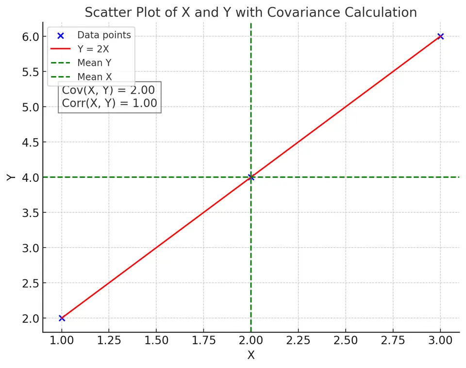
Let's calculate the covariance between two variables $X$ and $Y$ using the following dataset:
| Observation ($i$) | $X_i$ | $Y_i$ |
|---|---|---|
| 1 | 1 | 2 |
| 2 | 2 | 4 |
| 3 | 3 | 6 |
Step 1: Calculate the Sample Means
Compute the mean of $X$ and $Y$:
$$ \bar{X} = \frac{1}{n} \sum_{i=1}^{n} X_i = \frac{1 + 2 + 3}{3} = \frac{6}{3} = 2 $$
$$ \bar{Y} = \frac{1}{n} \sum_{i=1}^{n} Y_i = \frac{2 + 4 + 6}{3} = \frac{12}{3} = 4 $$
Step 2: Compute the Deviations from the Mean
Calculate $(X_i - \bar{X})$ and $(Y_i - \bar{Y})$:
| $i$ | $X_i$ | $Y_i$ | $X_i - \bar{X}$ | $Y_i - \bar{Y}$ |
|---|---|---|---|---|
| 1 | 1 | 2 | $1 - 2 = -1$ | $2 - 4 = -2$ |
| 2 | 2 | 4 | $2 - 2 = 0$ | $4 - 4 = 0$ |
| 3 | 3 | 6 | $3 - 2 = 1$ | $6 - 4 = 2$ |
Step 3: Calculate the Product of Deviations
Compute $(X_i - \bar{X})(Y_i - \bar{Y})$:
| $i$ | $X_i - \bar{X}$ | $Y_i - \bar{Y}$ | $(X_i - \bar{X})(Y_i - \bar{Y})$ |
|---|---|---|---|
| 1 | -1 | -2 | $(-1)(-2) = 2$ |
| 2 | 0 | 0 | $(0)(0) = 0$ |
| 3 | 1 | 2 | $(1)(2) = 2$ |
Step 4: Sum the Products of Deviations
Compute the sum:
$$ \sum_{i=1}^{n} (X_i - \bar{X})(Y_i - \bar{Y}) = 2 + 0 + 2 = 4 $$
Step 5: Calculate the Sample Covariance
Use the sample covariance formula:
$$ s_{XY} = \frac{1}{n - 1} \sum_{i=1}^{n} (X_i - \bar{X})(Y_i - \bar{Y}) $$
Since $n = 3$:
$$ s_{XY} = \frac{1}{3 - 1} \times 4 = \frac{1}{2} \times 4 = 2 $$
Interpretation:
- The positive covariance of $2$ indicates that $X$ and $Y$ tend to increase together.
- The table also shows $Y=2X$ exactly. Covariance by itself does not certify that a relationship is perfect: the value $2$ must be considered alongside $s_X=1$ and $s_Y=2$. Their product equals the covariance, giving the correlation of one calculated below.
Step 6: Calculate the Variances (Optional)
For completeness, calculate the variances of $X$ and $Y$:
Variance of $X$
$$ s_{XX} = \frac{1}{n - 1} \sum_{i=1}^{n} (X_i - \bar{X})^2 $$
Compute $(X_i - \bar{X})^2$:
| $i$ | $X_i - \bar{X}$ | $(X_i - \bar{X})^2$ |
|---|---|---|
| 1 | -1 | $(-1)^2 = 1$ |
| 2 | 0 | $(0)^2 = 0$ |
| 3 | 1 | $(1)^2 = 1$ |
Sum:
$$ \sum_{i=1}^{n} (X_i - \bar{X})^2 = 1 + 0 + 1 = 2 $$
Compute variance:
$$ s_{XX} = \frac{1}{2} \times 2 = 1 $$
Variance of $Y$
Similarly, compute $(Y_i - \bar{Y})^2$:
| $i$ | $Y_i - \bar{Y}$ | $(Y_i - \bar{Y})^2$ |
|---|---|---|
| 1 | -2 | $(-2)^2 = 4$ |
| 2 | 0 | $(0)^2 = 0$ |
| 3 | 2 | $(2)^2 = 4$ |
Sum:
$$ \sum_{i=1}^{n} (Y_i - \bar{Y})^2 = 4 + 0 + 4 = 8 $$
Compute variance:
$$ s_{YY} = \frac{1}{2} \times 8 = 4 $$
Step 7: Calculate the Correlation Coefficient (Optional)
The correlation coefficient $r_{XY}$ standardizes the covariance, providing a dimensionless measure of the strength and direction of the linear relationship:
$$ r_{XY} = \frac{s_{XY}}{\sqrt{s_{XX} \times s_{YY}}} = \frac{2}{\sqrt{1 \times 4}} = \frac{2}{2} = 1 $$
Interpretation:
- A correlation coefficient of $1$ indicates a perfect positive linear relationship between $X$ and $Y$.
- This makes sense since $Y = 2X$ in the dataset.
Plot:
Limitations of Covariance
I. Scale Dependence:
- Covariance values are affected by the units of measurement of the variables.
- For example, measuring height in meters vs. centimeters will change the covariance.
II. Comparison Difficulties:
- Because covariance is not standardized, comparing covariances across different datasets or variables with different scales is challenging.
- This is why the correlation coefficient, which standardizes covariance, is often used.
III. Not a Measure of Strength:
- The magnitude of covariance does not directly indicate the strength of the relationship.
- A large covariance could be due to large variances rather than a strong relationship.
- Covariance values are not bounded by a universal constant; only $|\text{Cov}(X,Y)|\le\sigma_X\sigma_Y$ holds.
IV. Linear Relationships Only:
- Covariance measures only linear relationships.
- It does not characterize general dependence. Some nonlinear relationships have nonzero covariance, while others have zero covariance because positive and negative products cancel. A scatterplot and the joint model provide information that covariance alone cannot supply.