Sequences and Series

A time-series model often says that today's observation contains the effects of many earlier shocks. Writing those effects as an infinite sum is convenient, but it raises a concrete question: does including more history settle on a definite answer, or does the approximation keep changing without limit?

Sequences and series supply the tools for answering that question. A sequence is the ordered list of terms; a series adds them. The terms of a sequence may approach zero while their sum still grows without bound, so these are separate convergence questions.

In a stable AR(1), a shock's weights are $1,\phi,\phi^2,\ldots$. Their decay determines how long the shock remains influential. In an inverse MA filter, similar powers determine whether the hidden shock can be recovered reliably from observations. Both uses require an infinite expression to be the limit of finite calculations.

For numerical terms, examine ordinary and absolute convergence. For sums of random shocks, also examine mean-square convergence: it measures whether the expected squared error from truncating the history tends to zero. These conditions justify different operations and should not be substituted for one another.

Worked calculation: a geometric series

Consider the terms

$$ 1,\quad0.5,\quad0.5^2,\quad0.5^3,\ldots $$

The partial sum through the fourth power is

$$ S_4=1+0.5+0.25+0.125+0.0625=1.9375. $$

The infinite sum is

$$ \sum_{j=0}^{\infty}0.5^j=\frac{1}{1-0.5}=2. $$

So the omitted tail after $S_4$ is

$$ 2-1.9375=0.0625. $$

The limit 2 tells us where the partial sums are heading; the tail 0.0625 tells us how far this particular approximation remains from that limit. In a time-series filter, knowing that the tail tends to zero is only the first step. To choose a usable truncation length, we need to know how quickly it shrinks and how large an omitted contribution we can tolerate.

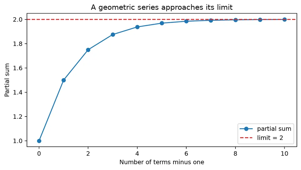
The figure shows the partial sums approaching 2. Each added term improves the approximation, but the size of the improvement shrinks because the geometric weights decay.

Sequences

A sequence is an ordered list of numbers, formally a function that maps an index such as a natural number $n$ to a value $a_n$:

$$ a_1,a_2,a_3,\dots,a_n,\dots $$

A sequence converges to $a$ if its terms become arbitrarily close to $a$ as $n$ increases:

$$ \lim_{n\to\infty}a_n=a. $$

Equivalently, for every $\epsilon>0$, there is an index $N$ such that

$$ |a_n-a|<\epsilon $$

for all $n>N$. If no finite limit satisfies this condition, the sequence diverges.

Examples of Sequences

A convergent example is

$$ a_n=\frac{n}{n+2}. $$

Its first terms are

$$ \frac13,\frac24,\frac35,\dots, $$

and

$$ \lim_{n\to\infty}\frac{n}{n+2}=1. $$

By contrast,

$$ a_n=4^n $$

grows without bound, so it diverges. The sequence

$$ a_n=n+1 $$

also diverges because its terms increase indefinitely.

Another convergent example is

$$ a_n=\frac{1}{n^3}, $$

for which

$$ \lim_{n\to\infty}\frac{1}{n^3}=0. $$

The examples so far concern individual terms. For $a_n=1/n$, the next term eventually becomes very small, but there are infinitely many terms still to add. Small terms therefore do not, by themselves, make a finite total. To study the total, construct a second sequence: the accumulated sums after one term, two terms, and so on.

Partial Sums

For a sequence $\{a_n\}$, the partial sum of the first $n$ terms is

$$ s_n=a_1+a_2+\dots+a_n. $$

Thus,

$$ s_1=a_1, \qquad s_2=a_1+a_2, \qquad s_3=a_1+a_2+a_3, $$

and so on. Infinite-series convergence is defined through the behavior of this sequence of partial sums.

Series

A series is the formal sum of the terms of a sequence. If the partial sums converge to a finite limit $s$, then

$$ \sum_{k=1}^{\infty}a_k =\lim_{n\to\infty}s_n =s. $$

If the partial sums do not approach a finite limit, the series diverges. Therefore, a term sequence approaching zero is necessary for series convergence but is not sufficient; the harmonic series later in the chapter is the standard counterexample.

Geometric Series and Rational Functions

A geometric series has the form

$$ \sum_{k=0}^{\infty}r^k. $$

When $|r|<1$,

$$ \sum_{k=0}^{\infty}r^k=\frac{1}{1-r}. $$

Equivalently,

$$ \frac{1}{1-x}=\sum_{k=0}^{\infty}x^k, \qquad |x|<1. $$

The rational expression $1/(1-x)$ and the infinite series describe the same quantity only within the stated convergence region. Substituting a lag operator into the formal algebra does not remove that restriction. For example, expanding $(1-\phi B)^{-1}$ gives a history with weights $\phi^j$; those weights decay when $|\phi|<1$. Outside that region, the same formal geometric expansion is not a stable past-based representation.

Examples of Convergent Series

A geometric series with ratio $1/3$ is

$$ \sum_{k=0}^{\infty}\frac{1}{3^k} =\frac{1}{1-1/3} =\frac32. $$

A p-series is

$$ \sum_{k=1}^{\infty}\frac{1}{k^p}. $$

It converges for $p>1$. In particular,

$$ \sum_{k=1}^{\infty}\frac{1}{k^2}=\frac{\pi^2}{6}. $$

An alternating series changes sign from term to term. The alternating harmonic series,

$$ \sum_{k=1}^{\infty}\frac{(-1)^{k+1}}{k}, $$

converges to

$$ \ln 2. $$

These examples illustrate different reasons for convergence: geometric decay, sufficiently fast polynomial decay, and cancellation in an alternating sequence.

Examples of Divergent Series

A geometric series with ratio larger than 1 in magnitude diverges. For example,

$$ \sum_{k=1}^{\infty}4^k=4+16+64+\dots $$

has partial sums that grow without bound.

An arithmetic-term series such as

$$ \sum_{k=1}^{\infty}(2k+3)=5+7+9+\dots $$

also diverges because the terms themselves do not approach zero.

The harmonic series

$$ \sum_{k=1}^{\infty}\frac{1}{k} =1+\frac12+\frac13+\dots $$

is more subtle. Its terms do approach zero, but the partial sums still grow without bound. This is why checking $a_n\to0$ is only a necessary condition for convergence.

Absolute Convergence

A series is absolutely convergent if

$$ \sum_{k=1}^{\infty}|a_k| $$

converges. Absolute convergence implies ordinary convergence. The converse is not always true: the alternating harmonic series converges, but the corresponding series of absolute values is the divergent harmonic series.

Absolute convergence prevents convergence from depending on delicate cancellation between positive and negative terms. If the input to a filter is bounded in magnitude by $M$, an absolutely summable coefficient sequence gives an output bounded by $M\sum_j|\psi_j|$. This is a useful deterministic notion of stability. For uncorrelated random inputs, the weaker requirement of square-summable coefficients can suffice for a finite output variance; the assumptions and the conclusion are different.

Convergence Tests

Choose a convergence test by the structure of the terms: positivity, alternation, geometric decay, or a useful comparison. The tests below examine the tail of the series, because changing finitely many initial terms cannot change whether the remaining infinite sum converges. For the ratio and root tests, a limiting value of 1 is inconclusive and requires another argument.

Integral test. Suppose $f(x)$ is positive, continuous, and decreasing for $x\ge1$, with $f(n)=a_n$. Then

$$ \sum_{n=1}^{\infty}a_n $$

and

$$ \int_1^{\infty}f(x)\,dx $$

converge or diverge together. For example, $\sum 1/n^2$ converges because

$$ \int_1^{\infty}\frac{1}{x^2}\,dx=1. $$

Comparison test. If

$$ 0\le a_n\le b_n $$

and $\sum b_n$ converges, then $\sum a_n$ also converges. For example,

$$ \frac{1}{n^3+2}<\frac{1}{n^3}, $$

and $\sum1/n^3$ is a convergent p-series, so

$$ \sum_{n=1}^{\infty}\frac{1}{n^3+2} $$

converges.

Limit comparison test. For positive-term series, if

$$ \lim_{n\to\infty}\frac{a_n}{b_n}=c, \qquad 0<c<\infty, $$

then $\sum a_n$ and $\sum b_n$ have the same convergence behavior. For

$$ a_n=\frac{n^2+1}{n^4+3}, \qquad b_n=\frac{1}{n^2}, $$

we have

$$ \lim_{n\to\infty} \frac{\frac{n^2+1}{n^4+3}}{\frac1{n^2}} = \lim_{n\to\infty}\frac{n^4+n^2}{n^4+3} =1. $$

Because $\sum1/n^2$ converges, so does the original series.

Alternating series test. For an alternating series

$$ \sum(-1)^na_n, $$

if $a_n\ge0$ decreases eventually and $a_n\to0$, then the series converges. The alternating harmonic series satisfies these conditions.

Ratio test. Let

$$ L=\lim_{n\to\infty}\left|\frac{a_{n+1}}{a_n}\right|. $$

If $L<1$, the series converges absolutely; if $L>1$, it diverges; if $L=1$, the test is inconclusive. For

$$ a_n=\frac{n!}{n^n}, $$

$$ \frac{a_{n+1}}{a_n} =\left(\frac{n}{n+1}\right)^n, $$

so

$$ L=e^{-1}<1. $$

Therefore the series converges.

Root test. Let

$$ L=\limsup_{n\to\infty}|a_n|^{1/n}. $$

If $L<1$, the series converges absolutely; if $L>1$, it diverges. For

$$ a_n=\left(\frac34\right)^n, $$

$$ L=\frac34<1, $$

so the geometric series converges.

Mean-Square Convergence

For random variables, convergence can be defined through expected squared error. A sequence $X_n$ converges to $X$ in mean square if

$$ E[(X_n-X)^2]\to0 \quad\text{as }n\to\infty. $$

Mean-square convergence treats a finite sum as an approximation to a random quantity and averages its squared error across possible realizations. It is stronger than checking whether one plotted realization happens to settle. If the omitted error has mean zero, its mean square is its variance, so a variance calculation often proves convergence directly. This is why second moments appear so frequently in proofs about infinite time-series filters.

Inverting the MA(1) Model

Consider

$$ X_t=Z_t+\beta Z_{t-1}, $$

where $Z_t$ is white noise with mean zero and variance $\sigma_Z^2$. Rearranging and repeatedly substituting gives

$$ Z_t=\sum_{k=0}^{\infty}(-\beta)^kX_{t-k}. $$

This inverse representation is stable when the geometric coefficients decay, which for MA(1) means

$$ |\beta|<1. $$

Autocovariance Function of the MA(1) Process

The autocovariance function is

$$ \gamma(k)= \begin{cases} (1+\beta^2)\sigma_Z^2, & k=0,\\ \beta\sigma_Z^2, & |k|=1,\\ 0, & |k|>1. \end{cases} $$

At lag 1, the two observations contain one common shock, producing the term $\beta\sigma_Z^2$. Beyond lag 1 they contain disjoint shock indices, so uncorrelated shocks give zero covariance. This finite covariance range belongs to the original MA(1) process. Its inverse filter can still require infinitely many observations: a short forward shock response does not imply a short inverse response.

Series Convergence in Mean-Square Sense

Consider the partial inverse

$$ S_n=\sum_{k=0}^{n}(-\beta)^kX_{t-k}. $$

Substitute the MA equation into every term of $S_n$. Each interior shock appears twice with opposite coefficients and cancels. The current shock $Z_t$ remains, together with one boundary shock from just beyond the retained history. Keeping that boundary term gives an exact finite identity, rather than assuming that an infinite expansion has already converged:

$$ Z_t =S_n+(-\beta)^{n+1}Z_{t-n-1}. $$

Therefore the truncation error is

$$ Z_t-S_n=(-\beta)^{n+1}Z_{t-n-1}, $$

and its mean square is

$$ E[(Z_t-S_n)^2] =\beta^{2(n+1)}\sigma_Z^2. $$

Condition for Convergence

Mean-square convergence requires

$$ \beta^{2(n+1)}\sigma_Z^2\to0, $$

which occurs exactly when

$$ |\beta|<1. $$

The remaining boundary shock has the same variance at every truncation length; only its coefficient changes. Consequently, the approximation improves precisely when that coefficient tends to zero. For a nondegenerate innovation variance, $|\beta|<1$ makes the squared error vanish, $|\beta|=1$ leaves it unchanged, and $|\beta|>1$ makes it grow. The invertibility condition is therefore visible in an actual approximation error, not only in a polynomial rule.

Invertibility Condition

The MA polynomial is

$$ \beta(B)=1+\beta B. $$

Its zero is

$$ B=-\frac{1}{\beta}. $$

Requiring that zero to lie outside the unit circle gives

$$ \left|-\frac{1}{\beta}\right|>1 \quad\Longleftrightarrow\quad |\beta|<1. $$

Invertibility therefore links a polynomial root condition, geometric-series convergence, and stable recovery of the innovations.

From convergent coefficients to a well-defined random process

Infinite series appear whenever a stable dynamic model is rewritten as a weighted history of shocks or observations. The geometric identity

$$ \sum_{j=0}^{\infty}r^j=\frac{1}{1-r}, \qquad |r|<1, $$

is the simplest example.

With $r=0.5$,

$$ S_4=1+0.5+0.25+0.125+0.0625=1.9375, \qquad S_\infty=2. $$

The omitted tail is

$$ \sum_{j=5}^{\infty}0.5^j =\frac{0.5^5}{1-0.5}=0.0625. $$

For a linear process

$$ X_t=\sum_{j=0}^{\infty}\psi_j\varepsilon_{t-j}, $$

square summability,

$$ \sum_{j=0}^{\infty}\psi_j^2<\infty, $$

ensures mean-square convergence and a finite variance when the shocks have mean zero, a common finite variance, and zero covariance across time. If $\psi_j=0.5^j$, then

$$ \sum_{j=0}^{\infty}0.25^j =\frac{1}{0.75} =\frac43. $$

Thus, if $\mathrm{Var}(\varepsilon_t)=\sigma^2$,

$$ \mathrm{Var}(X_t)=\frac43\sigma^2. $$

The variance uses squared weights because the variance of a weighted shock is its squared coefficient times the shock variance. Cross-products disappear because different shocks are uncorrelated. Thus the numerical sum of weights is 2 in the opening example, while the sum of squared weights is $4/3$ here. Confusing these two sums would give the wrong process variance even though both geometric series converge.

Numerical stability

Finite computations truncate infinite representations. For a geometric series with $|r|<1$, the absolute tail after retaining terms through $m$ satisfies

$$ \left|\sum_{j=m+1}^{\infty}r^j\right| =\frac{|r|^{m+1}}{|1-r|} $$

This is the exact absolute tail when $|r|<1$. A bound expressed only in terms of the magnitude $|r|$ is often more convenient. The triangle inequality gives

$$ \frac{|r|^{m+1}}{1-|r|} $$

This bound uses absolute coefficient magnitudes, so it applies whether the geometric weights keep one sign or alternate.

A coefficient close to 1 can make a valid infinite representation expensive to approximate. With $r=0.5$, each additional term halves the remaining geometric contribution. With $r=0.99$, each term reduces it by only about one percent. A fixed truncation length that works well in the first case can be inaccurate in the second. Choose the retained history from an error tolerance or sensitivity check, especially when interpreting a model with strong persistence.

Formula reference