Multiple Comparisons

When conducting multiple hypothesis tests, the probability of making at least one Type I error—falsely rejecting a true null hypothesis—increases. This is known as the multiple comparisons problem or, in some contexts, the look-elsewhere effect.

Methods for addressing this problem typically adjust significance thresholds or p-values. Different methods control different types of error and involve different trade-offs between false positives and statistical power.

Data Snooping and the Multiple Testing Fallacy

• A 1992 Swedish study reported a statistically significant association between living near power lines and childhood leukemia, but later studies did not consistently replicate the finding.
• The study examined a large number of possible associations, increasing the chance that some results would appear statistically significant by chance.
• The multiple testing fallacy occurs when many tests are performed without accounting for the increased chance of false positives. For example, if 800 independent null hypotheses are all true and each is tested at a 1% significance level, about 8 false positives would be expected on average.

Multiple Comparisons Problem

• A p-value is the probability, assuming the null hypothesis is true, of obtaining a result at least as extreme as the one observed. A smaller p-value indicates stronger evidence against the null hypothesis.
• The look-elsewhere effect refers to the increased chance of finding an apparently significant result when many possible comparisons are examined.
• Data snooping is the broader practice of repeatedly exploring data and then treating selected patterns as if they had been specified in advance.

Reproducibility and Replicability Crisis

• Reproducibility refers to obtaining the same results using the same data and analysis procedures, while replicability refers to obtaining consistent results in a new study using new data.
• Concerns about the reliability of published findings are often described as the reproducibility and replicability crisis. Practices such as extensive data exploration, selective reporting, and uncorrected multiple testing can contribute to this problem. John Ioannidis's 2005 paper, "Why Most Published Research Findings Are False," discusses several related issues.

Addressing the Multiple Testing Problem

• The Bonferroni correction controls the probability of making at least one Type I error across a family of tests. It can be implemented by dividing the desired family-wise significance level by the number of tests, or equivalently by multiplying each p-value by the number of tests. The method is simple but can be conservative, reducing statistical power.
• The false discovery proportion (FDP) is the proportion of rejected null hypotheses that are actually false discoveries. For example, if 80 true discoveries and 41 false discoveries are made, then the FDP is:

$$ \frac{41}{80+41}\approx0.34 $$

so about 34% of the reported discoveries are false positives.

False Discovery Rate (FDR)

• The false discovery rate (FDR) is the expected value of the false discovery proportion.
• The Benjamini-Hochberg procedure controls the FDR by ranking p-values and comparing them with thresholds that depend on their rank. It is generally less conservative than methods designed to control the family-wise error rate.

Using a Validation Set to Avoid Data Snooping

• The validation set approach divides the available data into separate sets so that exploratory findings can be evaluated on data that were not used to generate them.
• The model-building set is used to explore the data and identify possible relationships.
• The validation set is reserved for evaluating hypotheses or models that emerged during the exploratory phase.
• It is important that the validation set remain separate from the exploratory analysis. Repeatedly examining or tuning decisions based on the validation set can reintroduce data snooping.

Family-wise Error Rate (FWER)

The family-wise error rate (FWER) is the probability of making at least one Type I error among a defined family of hypothesis tests. Controlling FWER limits the probability of any false rejection within that family.

Bonferroni Correction

The Bonferroni correction is a common method for controlling the FWER. If the desired family-wise significance level is $\alpha$ and $m$ tests are performed, each individual test uses:

$$ \alpha_{\text{adjusted}} = \frac{\alpha}{m} $$

The Bonferroni correction is conservative, particularly when many tests are performed. This reduces the probability of false positives but can increase the probability of Type II errors, where a false null hypothesis is not rejected.

Example: Bonferroni Correction

Suppose we conduct 20 hypothesis tests and want to control the family-wise error rate at $\alpha = 0.05$. The Bonferroni-adjusted significance level is:

$$ \alpha_{\text{adjusted}} = \frac{\alpha}{m} = \frac{0.05}{20} = 0.0025 $$

where:

• $\alpha = 0.05$ is the desired family-wise significance level,
• $m = 20$ is the number of tests.

Conclusion:

After applying the Bonferroni correction, we reject the null hypothesis for an individual test only if its p-value is less than or equal to $0.0025$.

This controls the family-wise error rate at no more than 0.05, but the stricter threshold also reduces power and can increase the number of false negatives.

False Discovery Rate (FDR)

Unlike FWER, which controls the probability of making at least one false rejection, the false discovery rate controls the expected proportion of false discoveries among all rejected null hypotheses.

FDR-controlling procedures are generally more powerful than FWER-controlling methods, making them useful in exploratory settings where many hypotheses are tested and some false discoveries can be tolerated.

Benjamini-Hochberg Procedure

The Benjamini-Hochberg (BH) procedure controls the FDR by ordering the p-values from smallest to largest:

$$ p_{(1)} \leq p_{(2)} \leq \cdots \leq p_{(m)} $$

Each ordered p-value is compared with:

$$ \frac{i}{m}\alpha $$

where:

• $i$ is the rank of the p-value,
• $m$ is the total number of tests,
• $\alpha$ is the desired FDR level.

We find the largest rank $k$ such that:

$$ p_{(k)} \leq \frac{k}{m}\alpha $$

and reject the null hypotheses corresponding to:

$$ p_{(1)},\ldots,p_{(k)}. $$

Example: Multiple Hypothesis Testing

Suppose we conduct six hypothesis tests and obtain the p-values:

$$ \{0.001, 0.008, 0.039, 0.041, 0.042, 0.06\} $$

The following example uses the Holm-Bonferroni procedure, which controls the family-wise error rate rather than the false discovery rate.

We apply the procedure at $\alpha = 0.05$ by comparing each ordered p-value with a sequentially adjusted significance level.

Step-by-Step Procedure:

I. Order the p-values in ascending order:

$$ 0.001, 0.008, 0.039, 0.041, 0.042, 0.06 $$

II. Adjust the significance level for each test:

$$ \alpha_i = \frac{\alpha}{m-i+1} $$

where $m=6$ and $\alpha=0.05$.

III. Compare each p-value with its adjusted threshold:

For $p_1 = 0.001$:

$$ 0.001 < \frac{0.05}{6} \approx 0.00833 \quad \text{(Reject $H_0$)} $$

For $p_2 = 0.008$:

$$ 0.008 < \frac{0.05}{5} = 0.01 \quad \text{(Reject $H_0$)} $$

For $p_3 = 0.039$:

$$ 0.039 > \frac{0.05}{4} = 0.0125 \quad \text{(Fail to reject $H_0$)} $$

The Holm-Bonferroni procedure stops at the first hypothesis that is not rejected. Therefore, the remaining hypotheses are also not rejected.

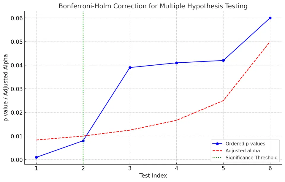
Using the Holm-Bonferroni procedure, we reject the first two null hypotheses and fail to reject the remaining four.

The procedure controls the family-wise error rate while generally being less conservative than the standard Bonferroni correction. As with other multiple-testing procedures, stronger protection against false positives comes at the cost of reduced power and a greater risk of failing to detect real effects.