Moving Average (MA) Models

A moving-average model explains an observation through a short history of shocks. A temporary disruption may affect today's measurement and leave a smaller effect tomorrow, then disappear. An MA(1) encodes that pattern with one current shock and one lagged shock; an MA($q$) extends the direct response through $q$ lags.

The shocks are not the past observations. They are unobserved inputs whose overlapping effects create dependence between observations. This distinction explains both the theoretical covariance cutoff and why estimating an MA model requires more than regressing the series on its observed lags.

The word “average” can be misleading: MA coefficients need not be positive or sum to 1. The equation is a weighted shock model, not necessarily a smoothing operation. A rolling mean or EMA instead transforms observed values into a smoothed series. Those operations appear later so that their inputs, outputs, and purposes can be compared directly with the stochastic MA equation.

Worked calculation: an MA(1)

Let

$$ X_t=\varepsilon_t+0.5\varepsilon_{t-1}, \qquad \mathrm{Var}(\varepsilon_t)=1. $$

Because the shocks are uncorrelated,

$$ \gamma(0)=1+0.5^2=1.25, \qquad \gamma(1)=0.5, \qquad \gamma(h)=0\quad(h>1). $$

Consequently,

$$ \rho(1)=\frac{0.5}{1.25}=0.4. $$

The theoretical ACF of this MA(1) cuts off after lag 1. In a finite sample, later sample autocorrelations will usually not be exactly zero.

Innovations and finite shock duration

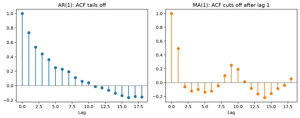
Moving-average (MA) models are a class of univariate time-series models in which the current value is a finite linear combination of current and past innovations. Unlike autoregressive models, they do not use past observed values directly in the model equation.

The name can be confusing: an MA($q$) stochastic model is not the same object as a rolling moving-average smoother. The distinction is made explicit later in the chapter.

Overview of Moving Average Models

An MA model represents short-lived shock effects. A new innovation can affect the current observation and the next few observations, but in an MA($q$) process its direct effect disappears after $q$ lags.

Two MA observations can be correlated only where their shock histories overlap, under uncorrelated shocks. Observations more than $q$ dates apart contain disjoint shock indices, giving covariance zero. With independent shocks, the separated observations are also independent. Under weak white noise alone, the covariance statement remains valid, but the stronger independence conclusion need not hold.

Mathematical Definition of MA Models

A moving average model of order $q$, MA($q$), can be written as

$$ Y_t=\mu+\varepsilon_t+\theta_1\varepsilon_{t-1}+\theta_2\varepsilon_{t-2}+\dots+\theta_q\varepsilon_{t-q}. $$

Equivalently, with $\theta_0=1$,

$$ Y_t=\mu+\sum_{i=0}^{q}\theta_i\varepsilon_{t-i}. $$

Here:

• $Y_t$ is the observation at time $t$;
• $\mu$ is the mean of the process under this parameterization;
• $\varepsilon_t$ is a white-noise innovation with mean zero and constant variance $\sigma^2$;
• $\theta_i$ is the coefficient on the innovation from lag $i$;
• $q$ is the largest innovation lag included directly in the model.

For the covariance calculations, we need zero-mean shocks with a common finite variance and zero covariance across dates. Independence is not necessary because the calculations use only second moments. A Gaussian likelihood or exact Gaussian prediction interval makes additional distributional assumptions. Distinguish the conditions needed to derive a covariance identity from those used to estimate or forecast probabilistically.

Examples of MA Models

First-Order Moving Average Model (MA(1))

An MA(1) includes the current innovation and one lagged innovation:

$$ Y_t=\mu+\varepsilon_t+\theta_1\varepsilon_{t-1}. $$

A shock at time $t$ therefore affects $Y_t$ and $Y_{t+1}$ directly, but not $Y_{t+2}$ or later observations.

Second-Order Moving Average Model (MA(2))

An MA(2) includes two lagged innovations:

$$ Y_t=\mu+\varepsilon_t+\theta_1\varepsilon_{t-1}+\theta_2\varepsilon_{t-2}. $$

A shock can affect three consecutive observations: the current one and the next two.

General MA($q$) Model

The general form is

$$ Y_t=\mu+\varepsilon_t+\theta_1\varepsilon_{t-1}+\dots+\theta_q\varepsilon_{t-q}. $$

The coefficients determine the magnitude and sign of the finite shock response.

Properties of MA Models

With fixed coefficients, the same finite combination of shocks is applied at every date. Its mean is therefore $\mu$, and its variance is $\sigma^2\sum_{j=0}^q\theta_j^2$ with $\theta_0=1$. All cross-terms vanish because different shocks are uncorrelated. The same overlap calculation gives a covariance depending only on lag, establishing weak stationarity. Invertibility concerns reversing this mapping and is a separate condition.

Theoretical Properties of MA(1) Model

For

$$ Y_t=\mu+\varepsilon_t+\theta_1\varepsilon_{t-1}, $$

with innovation variance $\sigma^2$,

$$ E(Y_t)=\mu, $$

and

$$ \mathrm{Var}(Y_t)=\sigma^2(1+\theta_1^2). $$

At lag 1,

$$ \rho_1=\frac{\theta_1}{1+\theta_1^2}, $$

while for $|h|\ge2$,

$$ \rho_h=0. $$

At lag 1, the shared shock appears with coefficient 1 in one observation and $\theta_1$ in the other, giving covariance $\theta_1\sigma^2$. At lag 2 there is no shared shock index, so covariance is zero. Dividing by the variance yields the ACF. The cutoff is exact for the population process; estimated correlations from a finite sample fluctuate and will not form a perfectly zero tail.

Autocorrelation Function (ACF) in MA Models

For an MA($q$), the theoretical autocovariance is exactly zero for $|h|>q$. Lags at or below $q$ can be nonzero, although particular coefficient combinations can make some of them vanish as well.

Typical identification patterns are therefore:

• MA(1): the ACF can be nonzero at lag 1 and is zero after lag 1;
• MA(2): the ACF can be nonzero through lag 2 and is zero after lag 2;
• MA($q$): the ACF cuts off after lag $q$.

The PACF usually tails off rather than cutting off sharply. These are ideal population patterns and should be treated as heuristics in finite samples.

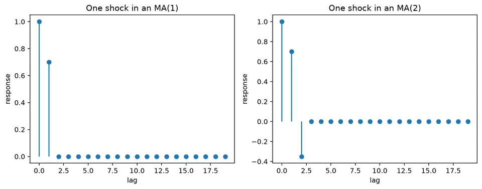
The figure shows the mechanism behind the cutoff: a single innovation has a finite sequence of direct effects and then disappears from the model equation.

Identifying the Order $q$ of an MA Model

A possible cutoff suggests how far the direct shock response might extend. It is only a proposal because sampling noise can create isolated later spikes, and trend or a break can create a broad correlation pattern unrelated to a finite MA mechanism. Fit a small range of plausible orders, use consistent data and likelihood conventions, and check what serial structure remains in the estimated innovations.

Step-by-Step Process for Model Selection

A practical sequence is:

1. plot the ACF and look for a plausible cutoff;
2. use uncertainty bands, such as the rough white-noise reference $\pm1.96/\sqrt n$, as screening guidance rather than an exact order rule;
3. fit a small set of candidate MA orders;
4. compare information criteria using the same response data and likelihood convention;
5. inspect residual autocorrelation and out-of-sample forecasts.

AIC and BIC are

$$ \mathrm{AIC}=-2\ln(L)+2k, $$

and

$$ \mathrm{BIC}=-2\ln(L)+k\ln(n), $$

where $L$ is the maximized likelihood, $k$ is the number of estimated parameters under the chosen convention, and $n$ is the sample size. Lower values are preferred within a comparable candidate set.

Example: Selecting an MA(2) Model

Suppose the sample ACF has notable spikes at lags 1 and 2 and no clear signal at later lags. That pattern suggests including MA(2) among the candidates.

If the fitted models give

then both criteria favor MA(2) among these three models. The remaining step is to verify that its residuals no longer contain systematic dependence and that its forecasts are competitive.

Example: Moving Average (MA) Model

Consider

$$ Y_t=\mu+w_t+\theta_1w_{t-1}, $$

with

• $\mu=10$,
• $\theta_1=0.5$,
• $w_t$ independent normal with mean 0 and variance 1.

The model is

$$ Y_t=10+w_t+0.5w_{t-1}. $$

Defining the MA(1) Model

The mean is 10 because both shocks have expectation zero; no averaging of past observations is being performed. If the current shock is zero and the previous shock was 2, today's value is $10+0+0.5(2)=11$. Tomorrow that previous shock has left the two-term equation. This makes the meaning of the lagged-shock coefficient concrete without treating the shock as an observed predictor.

Theoretical Autocorrelation Function (ACF) of MA(1)

For $\theta_1=0.5$,

$$ \rho_1=\frac{0.5}{1+0.5^2}=\frac{0.5}{1.25}=0.4, $$

and

$$ \rho_h=0\quad\text{for }|h|\ge2. $$

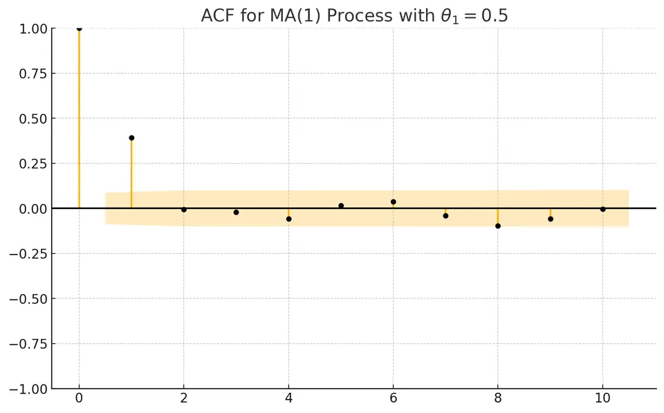
The first-lag spike represents the shared innovation between adjacent observations. Higher-lag population correlations are zero because observations more than one period apart share no innovation in an MA(1). A sample plot will show small nonzero values at later lags because of sampling variation.

Simple Moving Average (SMA)

A simple moving average (SMA) is a smoother, not an MA($q$) stochastic model. It takes the arithmetic mean of the most recent $k$ observed values:

$$ \mathrm{SMA}_t=\frac{1}{k}\sum_{i=0}^{k-1}y_{t-i}. $$

The smoother can be calculated directly once the window is chosen. A given observed value enters several neighboring smoothed outputs and then leaves the window. This overlap creates dependence in the smoothed series even if the original observations were independent. That fact helps explain the terminology, but it does not mean that fitting a latent-shock MA model is equivalent to applying a rolling mean to the data.

Exponential Moving Average (EMA)

An exponential moving average (EMA) is another smoothing rule. It updates a level recursively:

$$ \mathrm{EMA}_t=\alpha y_t+(1-\alpha)\mathrm{EMA}_{t-1}, $$

where $0<\alpha<1$. Larger values of $\alpha$ place more weight on the newest observation and make the smoother respond more quickly to recent changes.

Again, this is conceptually different from an MA($q$) stochastic model: an EMA is a deterministic transformation of observed data once $\alpha$ and the initial value are fixed.

Example: Stock Price Analysis

SMA and EMA curves are often plotted with price series as descriptive technical indicators. Their role is to summarize recent levels at different degrees of responsiveness; they do not, by themselves, provide a probabilistic model for future prices.

SMA Analysis

For a 20-day SMA,

$$ \mathrm{SMA}_t=\frac{P_t+P_{t-1}+\cdots+P_{t-19}}{20}. $$

Each price receives weight $1/20$ while it remains in the 20-day window, then its weight drops to zero. A new price replaces the oldest one, so the change in the SMA depends on both. After a sudden permanent rise, the smoother adjusts over several dates as older prices leave the window. The lag is a property of that averaging rule, not evidence of a delayed causal response in prices.

EMA Analysis

A commonly used EMA smoothing factor for a nominal span $N$ is

$$ \alpha=\frac{2}{N+1}. $$

The recursion is

$$ \mathrm{EMA}_t=\alpha P_t+(1-\alpha)\mathrm{EMA}_{t-1}. $$

Under this common span convention, the EMA emphasizes recent prices and gives a decaying weight to older prices rather than dropping them at a fixed window boundary. It can react more quickly to some changes than the corresponding SMA, but the exact comparison depends on the parameter, initialization, and price path.

Trend Identification

Practitioners sometimes interpret crossings or divergence between SMA and EMA curves as descriptive signals of changing momentum. Such rules depend on the chosen windows and should not be treated as guaranteed forecasts. Both curves are functions of past and current prices, so their usefulness must be evaluated against an explicit benchmark and out-of-sample data.

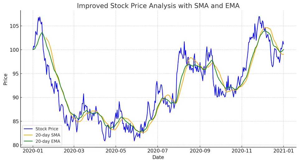
The figure shows the raw price path together with a 20-day SMA and EMA. The SMA is smoother and typically slower to react, while the EMA follows recent movements more closely. These curves illustrate smoothing behavior, not the innovation structure of an MA($q$) model.

From a shock response to estimation and identification

An MA($q$) model describes the current value as a finite weighted sum of current and past innovations:

$$ y_t=\mu+\varepsilon_t+\theta_1\varepsilon_{t-1}+\cdots+\theta_q\varepsilon_{t-q}. $$

The model inputs are current and lagged shocks rather than observed lags of the response. That difference explains both the finite shock-response pattern and the estimation problem: past shocks must be inferred from the observed series. Under the usual invertibility convention, they can be recovered by a stable past-based filter.

MA(1) numerical moments

Let

$$ y_t=\varepsilon_t+0.5\varepsilon_{t-1}, \qquad \mathrm{Var}(\varepsilon_t)=1. $$

Then

$$ \gamma(0)=1+0.5^2=1.25, \qquad \gamma(1)=0.5, \qquad \gamma(h)=0\quad(h>1). $$

Therefore,

$$ \rho(1)=\frac{0.5}{1.25}=0.4. $$

If a single shock $\varepsilon_t=2$ arrives and all other recent shocks are zero, its effect is 2 at time $t$, 1 at time $t+1$, and zero at $t+2$. The finite duration is the source of the theoretical ACF cutoff.

MA(2) response

For

$$ y_t=\varepsilon_t+0.7\varepsilon_{t-1}-0.35\varepsilon_{t-2}, $$

a shock of size 1 produces responses

$$ 1,\quad0.7,\quad-0.35,\quad0,\ldots $$

A positive shock can be followed by a positive contribution at the next date and a negative contribution at the date after that, depending on the MA coefficients. Thus a finite response need not decay smoothly or keep one sign. The response ends after lag 2 in this example because no later coefficient contains that shock. The covariance cutoff follows from the same finite-overlap mechanism.

Estimation

In AR estimation, an older observed value is already in the dataset. In MA estimation, the required older shock depends on the candidate parameters and on the reconstruction of previous shocks. Changing a coefficient therefore changes an entire inferred innovation sequence. Likelihood, innovations, and state-space methods account for this recursion instead of pretending that those shock lags are fixed observed regressors.

The treatment of initial innovations can matter in short series, so record the estimation method and software convention when reproducing fitted parameters.

Invertibility and equivalence

Different MA coefficient values can generate the same second-order autocovariance structure. Invertibility selects a unique representation whose inverse filter is stable. For an MA(1) written as

$$ (1+\theta B)\varepsilon_t, $$

the usual invertibility condition is $|\theta|<1$.

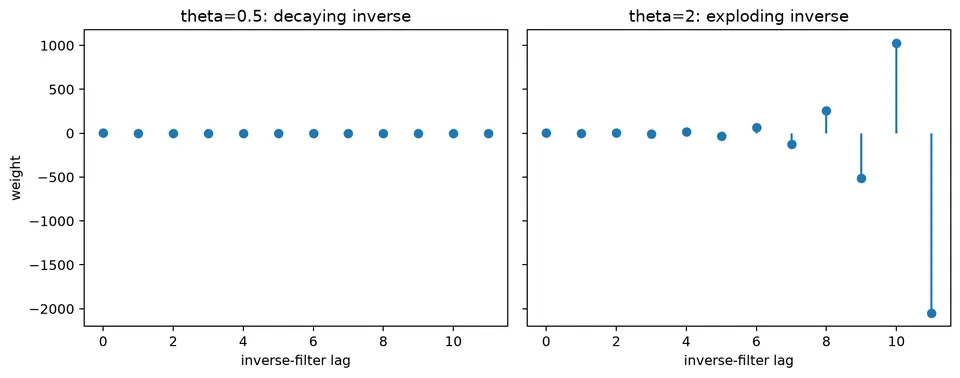
The figure illustrates why invertibility matters for identification: the observable covariance pattern can correspond to more than one coefficient representation unless a root convention is imposed.

MA versus moving-average smoother

Keep these three objects distinct:

The distinction can be checked by naming the input. The SMA and EMA take the observed series as input and produce a smoothed level. An MA model takes a hypothetical shock sequence as input and produces observations; estimation works backward to infer the shocks and coefficients. Using a smoother may improve a plot, but it does not by itself estimate that probabilistic shock-generating equation.

Formula reference