Stationarity in Time Series
Stationarity describes which probabilistic features of a time series remain stable when the time origin is shifted. Weak stationarity focuses on a constant mean and variance together with an autocovariance that depends only on lag, while strict stationarity requires the full joint distribution to be invariant to time shifts.
Many classical ARMA calculations rely on this stability because it lets dependence learned in one part of the series remain meaningful elsewhere. Trends, unit roots, seasonality, structural breaks, and changing variance violate stationarity in different ways, so the appropriate response may be detrending, differencing, seasonal modeling, variance transformation, or a model that explicitly allows change.
Formula reference
| Concept / case | General formula | Condition / interpretation |
|---|---|---|
| Strict stationarity | $(X_{t_1},\ldots,X_{t_k})\overset d=(X_{t_1+h},\ldots,X_{t_k+h})$ | Holds for every finite set of times and every common shift $h$. |
| Weak stationarity: mean | $E[X_t]=\mu$ | Constant over time. |
| Weak stationarity: variance | $\mathrm{Var}(X_t)=\gamma(0)<\infty$ | Constant finite variance. |
| Weak stationarity: covariance | $\mathrm{Cov}(X_t,X_{t-h})=\gamma(h)$ | Depends only on lag, not calendar time. |
| ACF | $\rho(h)=\gamma(h)/\gamma(0)$ | For a stationary process, $\rho(-h)=\rho(h)$. |
| White noise | $E\varepsilon_t=0$, $\mathrm{Var}(\varepsilon_t)=\sigma^2$, $\gamma(h)=0$ for $h\ne0$ | Basic stationary reference process. |
| MA($q$) covariance (with $\theta_0=1$) | $\gamma(h)=\sigma_\varepsilon^2\sum_{j=0}^{q-\lvert h\rvert}\theta_j\theta_{j+\lvert h\rvert}$ for $\lvert h\rvert\le q$ | Zero for $\lvert h\rvert>q$. |
| AR(1) | $X_t=c+\phi X_{t-1}+\varepsilon_t$ | Standard causal stationary solution requires $\lvert\phi\rvert<1$. |
| AR(1) mean | $\mu=c/(1-\phi)$ | Valid for the stationary solution. |
| AR(1) variance | $\gamma(0)=\sigma_\varepsilon^2/(1-\phi^2)$ | Finite only when $\lvert\phi\rvert<1$. |
| AR(1) ACF | $\rho(h)=\phi^{\lvert h\rvert}$ | Geometric or alternating decay. |
| AR($p$) stationarity/causality | $\phi(z)=1-\phi_1z-\cdots-\phi_pz^p=0\Rightarrow \lvert z\rvert>1$ | Standard backshift-root condition. |
| Linear filter | $X_t=\sum_j\psi_jY_{t-j}$ | Absolute summability $\sum_j\lvert\psi_j\rvert<\infty$ is a strong stability condition. |
| Random walk | $X_t=X_{t-1}+\varepsilon_t$ | Unit-root boundary; $\mathrm{Var}(X_t\mid X_0)=t\sigma^2$. |
| First difference | $\Delta X_t=(1-B)X_t=X_t-X_{t-1}$ | Removes one unit-root factor; a random walk becomes white noise. |
| Seasonal difference | $\Delta_sX_t=(1-B^s)X_t=X_t-X_{t-s}$ | Removes one seasonal unit-root factor at period $s$. |
| ADF regression | $\Delta X_t=\alpha+\beta t+\gamma X_{t-1}+\sum_{i=1}^{p}\delta_i\Delta X_{t-i}+\varepsilon_t$ | Unit-root null: $H_0:\gamma=0$. |
| KPSS decomposition | $X_t=d_t+r_t+u_t$, $r_t=r_{t-1}+\eta_t$ | Stationarity null corresponds to zero random-walk variance, $\mathrm{Var}(\eta_t)=0$. |
| Box-Cox transform | $g_\lambda(x)=(x^\lambda-1)/\lambda$ for $\lambda\ne0$; $g_0(x)=\log x$ | Used mainly to stabilize level-dependent variance, not to remove a unit root by itself. |
Worked calculation: the stationary AR(1) mean and variance
Consider
$$ X_t=1+0.8X_{t-1}+\varepsilon_t, \qquad \mathrm{Var}(\varepsilon_t)=1. $$
The stationary mean solves
$$ \mu=1+0.8\mu \quad\Longrightarrow\quad \mu=5. $$
After centering around 5, the stationary variance is
$$ \mathrm{Var}(X_t) =\frac{1}{1-0.8^2} =\frac{1}{0.36} \approx2.778. $$
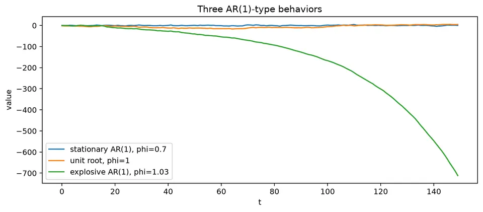
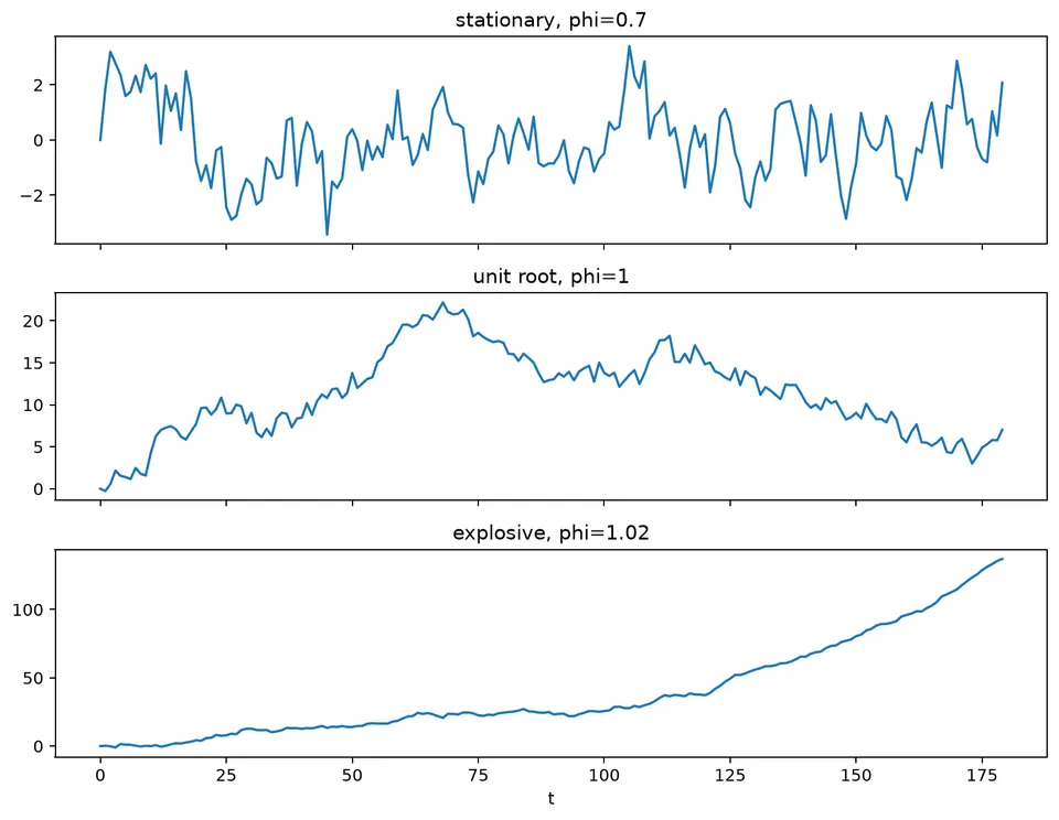
The calculation requires $|0.8|<1$. At $\phi=1$, the process is on the unit-root boundary and its variance does not settle to a finite constant. For $|\phi|>1$, deviations grow rather than decay.
The figure below contrasts these cases. A stationary AR(1) fluctuates around a stable level, a unit-root process wanders as shocks accumulate, and an explosive process moves increasingly far from its starting region.
Stationarity describes which probabilistic features of a time series remain stable as time shifts. For weak stationarity, the mean and variance are constant and autocovariance depends only on lag. This condition matters because ARMA models are formulated for stationary series, while ARIMA models handle certain non-stationary series by differencing them before applying an ARMA structure.
Two common definitions are used:
- Strict stationarity requires the entire joint distribution to be unchanged by a shift in time.
- Weak, or second-order, stationarity requires a constant mean and variance and an autocovariance that depends only on lag.
Why Do We Care About Stationarity?
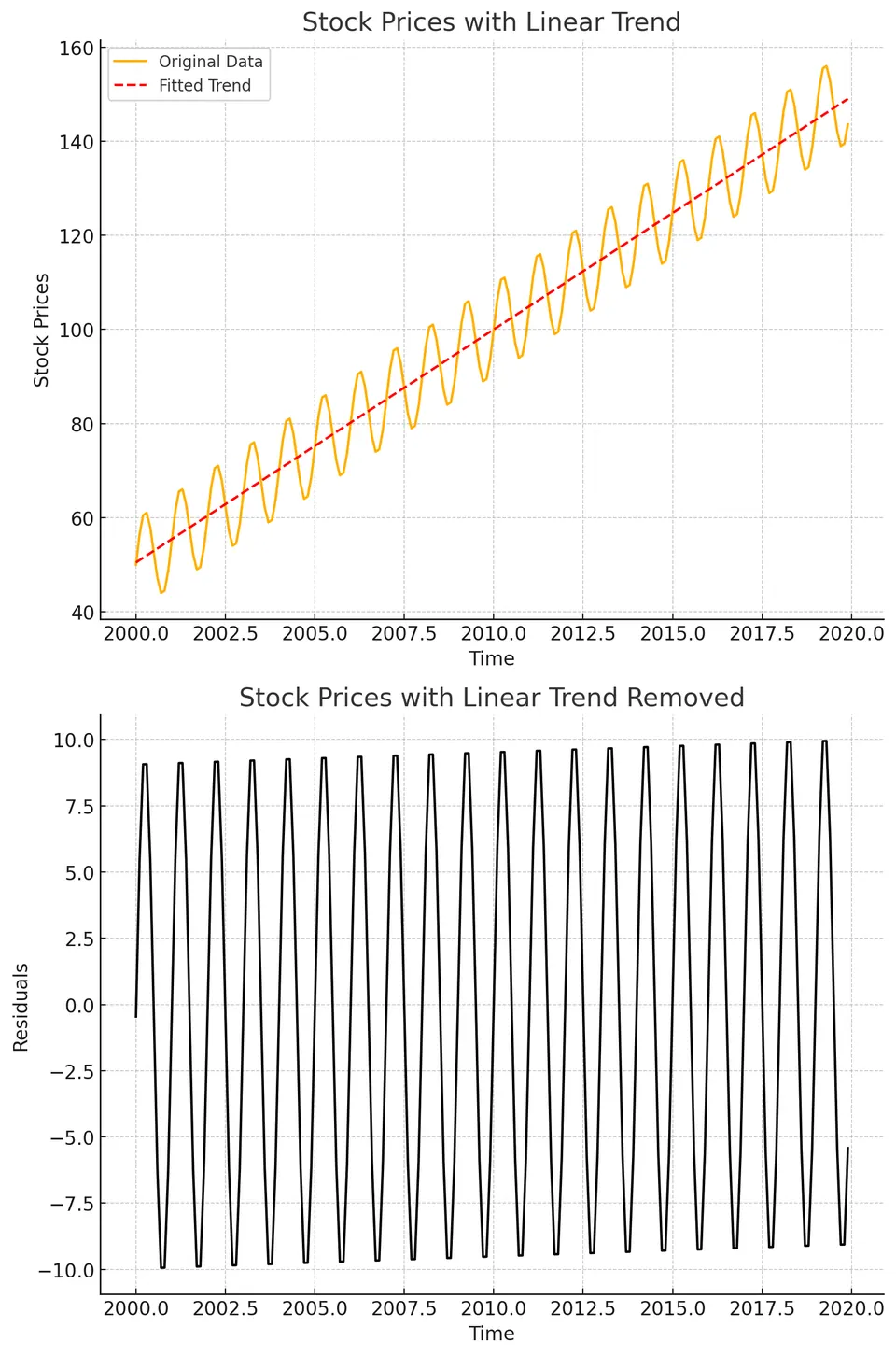
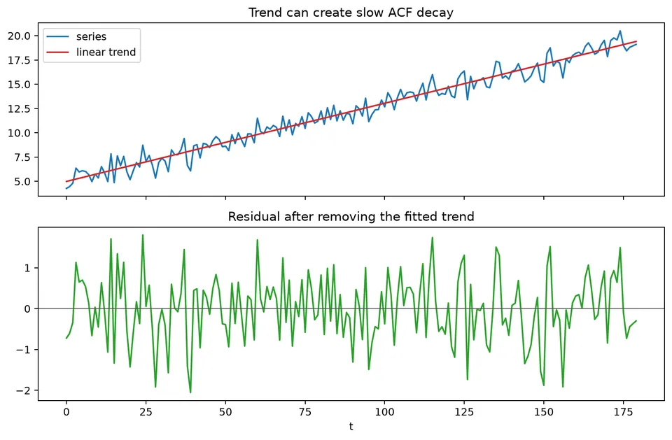
Suppose synthetic stock prices contain an upward deterministic trend together with shorter-term fluctuations, and the goal is to study recurring seasonal variation. The changing level can obscure that seasonal structure, so the mean pattern should be addressed before interpreting the remaining dependence.
Addressing non-stationarity by detrending
If a linear trend is a reasonable description of the changing mean, it can be estimated by least squares:
$$ \text{Stock Price} = z + b \times \text{Time}. $$
Here, $z$ is the intercept and $b$ is the slope. Subtracting the fitted trend gives residuals that fluctuate around the estimated mean structure. If the trend specification is appropriate, those residuals are better suited to studying seasonality and short-run dependence.
The next figure shows this progression: the upper panel contains the original series and fitted trend, while the lower panel shows the detrended residuals. The key point is that detrending changes the mean structure; it does not automatically guarantee stationarity.
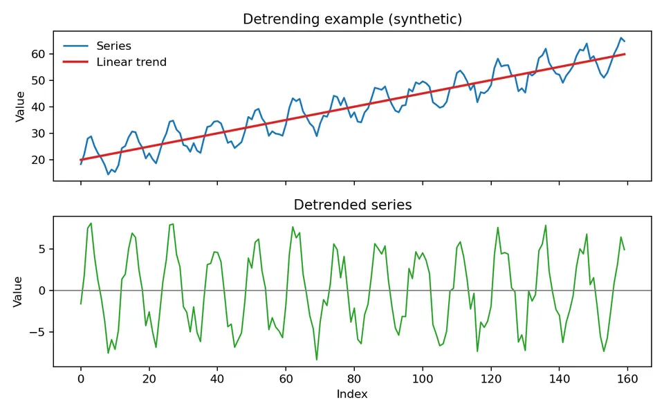
The following examples provide two additional views of detrending and its effect on the series.
Intuition for Stationary Time Series
A stationary series has a stable probabilistic structure over time. For weak stationarity:
- the mean does not systematically change with time;
- the variance remains constant; and
- dependence between observations is determined by their lag, not by their absolute position in time.
Deterministic trends or seasonal means violate these conditions. A stationary process can still show persistent or oscillating dependence through its autocovariance function, so stationarity does not mean that the series must look like featureless noise. Stability allows relationships estimated from one part of the series to remain relevant in another part.
Strict Stationarity
A process is said to be strictly stationary if the joint distribution of any subset of observations $X_{t_1}, X_{t_2}, \dots, X_{t_k}$ is the same as the distribution of $X_{t_1 + \tau}, X_{t_2 + \tau}, \dots, X_{t_k + \tau}$ for all $\tau$.
In simple terms, the process has the same probabilistic behavior after any common shift in time. Therefore the marginal distribution of $X_t$ does not change with $t$, and any moments that exist—such as the mean, variance, or higher moments—are also time-invariant.
Weak (Second-Order) Stationarity
Weak stationarity, also known as second-order stationarity, requires only a constant mean, a constant finite variance, and an autocovariance that depends solely on the lag between observations, not on time itself.
A time series $\{X_t\}$ is weakly stationary if:
- The mean of the series is constant: $E[X_t] = \mu$ for all $t$.
- The variance is constant: $\mathrm{Var}(X_t) = \sigma^2$ for all $t$.
- The autocovariance between $X_t$ and $X_{t+k}$ depends only on the lag $k$, not on $t$:
$$ \mathrm{Cov}(X_t, X_{t+k}) = \gamma(k) $$
Weak stationarity is the condition used in many classical time-series calculations because it makes means, variances, autocovariances, and correlations comparable across time.
Properties of Stationary Processes
Mean, Variance, and Autocovariance Functions
To analyze a stationary process, we focus on three key functions:
- The mean function $\mu(t) = E[X_t]$ represents the expected value of the process at time $t$, and for a stationary process, this should remain constant.
- The variance function $\sigma^2(t) = \mathrm{Var}(X_t)$ gives the variance at time $t$, which must also be constant for stationarity.
- The autocovariance function $\gamma(k) = \mathrm{Cov}(X_t, X_{t+k})$ measures how the process correlates with itself at different time lags $k$, and for a stationary process, it depends only on the lag $k$, not on time $t$.
More generally, the covariance function can be written as:
$$ \gamma(r, s) = \mathrm{Cov}(X_r, X_s) $$
Weak stationarity implies $\mu(t) = \mu$ and $\gamma(r, s)$ depends only on the lag $h = s - r$.
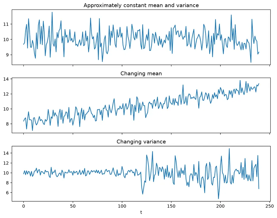
The figure below illustrates the contrast between stable moments and moments that change over time. Changes in the local mean or variance are visual evidence against global weak stationarity.
Autocorrelation and Bounds
For a weakly stationary process, the autocorrelation function $\rho(k)$, which measures the correlation between two points in the series separated by lag $k$, is bounded by -1 and 1:
$$ -1 \leq \rho(k) \leq 1 $$
This bound can be derived from basic linear algebra principles that apply to correlations between random variables.
q-Dependence and q-Correlation
A stationary series is q-dependent if observations separated by more than $q$ time units are independent. IID noise is therefore 0-dependent. An MA($q$) process driven by independent innovations is q-dependent, but general short-memory models such as AR and ARMA processes need not become independent after any finite lag.
A weaker property is q-correlation: the autocovariance is zero beyond lag $q$:
$$ \gamma(h) = 0 \quad \text{for} \quad |h| > q. $$
White noise is 0-correlated, and an MA($q$) process is q-correlated. Zero autocovariance does not by itself imply independence unless additional assumptions apply. Under standard second-order conditions, a stationary process with an autocovariance that cuts off after lag $q$ admits an MA($q$)-type second-order representation.
Linear Processes and Linear Filters
If $\{Y_t\}$ is a stationary series with mean 0 and autocovariance $\gamma_Y$, then a linear filter:
$$ X_t = \sum_{j=-\infty}^{\infty} \psi_j Y_{t-j} = \psi(B) Y_t $$
is also stationary when $\sum_{j=-\infty}^{\infty} |\psi_j| < \infty$. Many ARMA models can be viewed as linear filters applied to white noise.
The autocovariance of the filtered process is:
$$ \gamma_X(h) = \sum_{j=-\infty}^{\infty} \sum_{k=-\infty}^{\infty} \psi_j \psi_k\, \gamma_Y(h - k + j) $$
Examples of Stationary Processes
IID Noise vs. White Noise
IID noise with mean 0 and variance $\sigma^2$ is the simplest stationary building block. White noise is slightly weaker: it only requires zero mean and zero autocovariance for nonzero lags (uncorrelated), not full independence.
White Noise
White noise is a basic stationary building block. In the weak white-noise definition, the process has mean zero, constant finite variance, and zero autocovariance at every nonzero lag. Independence and Gaussianity are stronger assumptions, not part of the basic second-order definition. A common special case is Gaussian white noise, for which
$$ X_t \sim \mathcal{N}(0, \sigma^2). $$
Its second-order properties are:
- the mean is $E[X_t]=0$;
- the variance is $\mathrm{Var}(X_t)=\sigma^2$;
- the autocovariance function is:
$$ \gamma(k) = \begin{cases} \sigma^2 & \text{if } k = 0 \\ 0 & \text{if } k \neq 0 \end{cases} $$
- the autocorrelation function is:
$$ \rho(k) = \begin{cases} 1 & \text{if } k = 0 \\ 0 & \text{if } k \neq 0 \end{cases} $$
Below is a plot of synthetically generated white noise:
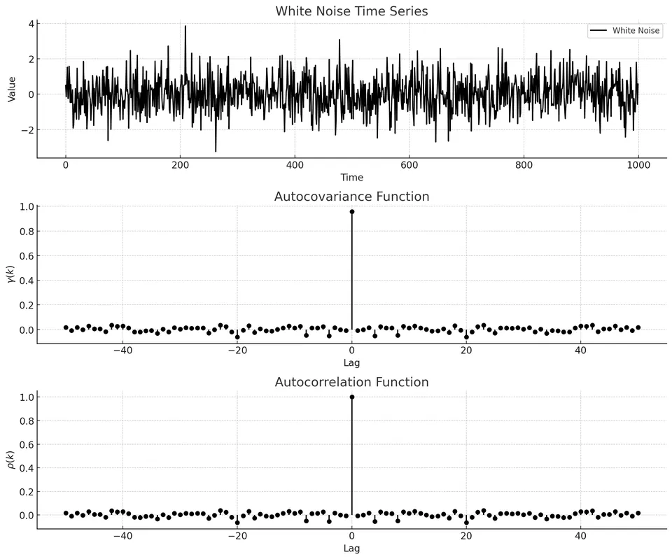
These properties make weak white noise weakly stationary. Gaussian white noise is also strictly stationary because its joint Gaussian distribution is determined by the constant mean and lag-based covariance structure.
Moving Average (MA) Process
A moving average process of order $q$, denoted MA($q$), is another weakly stationary model. It is defined as:
$$ X_t = \beta_0 Z_t + \beta_1 Z_{t-1} + \dots + \beta_q Z_{t-q} $$
where $Z_t$ is independent white noise with variance $\sigma_Z^2$; Gaussian innovations are a common special case.
For an MA(q) process:
- The mean is zero: $E[X_t] = 0$.
- The variance is constant:
$$ \mathrm{Var}(X_t) = \sigma_Z^2 \sum_{i=0}^{q} \beta_i^2 $$
- The autocovariance function $\gamma(k)$ depends on the lag $k$:
$$ \gamma(k) = \begin{cases} \sigma_Z^2 \sum_{i=0}^{q-|k|} \beta_i \beta_{i+|k|}, & |k| \leq q, \\ 0, & |k| > q. \end{cases} $$
The autocorrelation function $\rho(k)$ is obtained by normalizing the autocovariance by the variance:
$$ \rho(k) = \frac{\gamma(k)}{\gamma(0)} $$
The following plot shows an MA(2) realization. Its values can look locally dependent even though the theoretical autocovariance is exactly zero beyond lag 2:
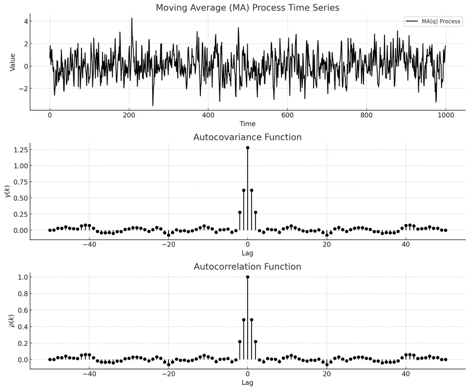
The MA(q) process is weakly stationary because its mean and variance are constant, and the autocovariance depends only on the lag.
Non-Stationary Processes
A non-stationary process does not satisfy the relevant stationarity conditions. Its mean, variance, dependence structure, or broader distribution may change over time. Deterministic trends, stochastic trends, seasonal means, structural breaks, and time-varying volatility are common sources.
Two important forms of non-stationarity are:
- trend-stationary processes;
- difference-stationary processes.
Trend-Stationary Processes
A trend-stationary series has a stable long-term trend around which the data fluctuates. If a time series follows a trend-stationary process, it tends to revert to its trend line after experiencing a disturbance.
Detrending.
To achieve stationarity in such series, one can remove the trend component. This is typically done by fitting a trend line (e.g., linear or polynomial) to the data and subtracting it from the original series. The resulting series, with the trend removed, should exhibit stationary behavior.
Difference-Stationary Processes
A difference-stationary series contains a stochastic trend, typically associated with a unit root. Subtracting a deterministic trend does not remove this accumulated effect of past shocks; differencing is used instead.
Differencing.
Taking differences between consecutive observations, or seasonal differences between observations one cycle apart, can remove an appropriate stochastic trend. The resulting series describes changes rather than levels and should be checked again for stationarity.
Transformations to Achieve Stationarity
To prepare a non-stationary time series for modeling with techniques that require stationarity (like ARIMA), various transformations can be applied:
Differencing
- Differencing can remove a stochastic trend and stabilize the mean when the integration structure justifies it.
- It involves computing the difference between consecutive observations in the series.
- The first difference of a series $Y_t$ is defined as $\Delta Y_t = Y_t - Y_{t-1}$.
- Higher-order differencing can be applied if trends persist, such as the second difference $\Delta^2 Y_t = \Delta Y_t - \Delta Y_{t-1}$.
- Use the smallest differencing order that produces an adequately stationary series; unnecessary differencing can create additional dependence.
Logarithmic Transformations
- Logarithmic transformations stabilize variance when variability increases with the magnitude of the data.
- The natural logarithm (or another logarithm base) is applied to each data point in the series.
- For a series $Y_t$, the transformed series becomes $\log(Y_t)$.
- This method is particularly effective for data exhibiting exponential growth or multiplicative seasonality.
- It also compresses large values, which can make proportional changes easier to compare.
Box-Cox Transformations
The Box-Cox transform generalizes the log transform for positive series:
$$ Y_t^{(\lambda)} = \begin{cases} \frac{Y_t^{\lambda} - 1}{\lambda}, & \lambda \neq 0 \\ \log(Y_t), & \lambda = 0 \end{cases} $$
Choosing $\lambda$ can stabilize variance and improve linearity before modeling.
Detrending
- Detrending removes long-term trends from data to highlight short-term fluctuations.
- A trend line is fitted to the data and then subtracted from the original series.
- For a linear trend $Y_t = \alpha + \beta t + \epsilon_t$, the detrended series is computed as $Y_t - (\alpha + \beta t)$.
- Non-linear trends can be removed by fitting polynomial or exponential functions.
- Detrending helps in isolating cyclical or seasonal patterns from broader trends.
The Random Walk Model
A random walk is a classic difference-stationary process. Each value equals the previous value plus a new innovation, so shocks accumulate permanently in the level of the series.
Definition
A random walk can be mathematically expressed as:
$$ X_t = X_{t-1} + Z_t $$
where $Z_t$ is an uncorrelated innovation sequence with mean $\mu_Z$ (zero for strict white noise, nonzero for a random walk with drift) and variance $\sigma_Z^2$. For a fixed starting value $X_0$, repeated substitution gives $X_t=X_0+\sum_{j=1}^t Z_j$.
Properties of a Random Walk
Mean. With fixed $X_0$,
$$ E[X_t] = X_0 + t\mu_Z. $$
For the common zero-drift random walk, $\mu_Z=0$, so the mean remains at $X_0$.
Variance. If the innovations are uncorrelated,
$$ \mathrm{Var}(X_t) = t\sigma_Z^2. $$
Thus even a zero-drift random walk is non-stationary: its variance increases with time, and shocks have permanent effects on the level.
Transforming a Random Walk into a Stationary Series
To utilize statistical models that require stationarity, it's necessary to transform a random walk into a stationary series. This is achieved through differencing.
Differencing Operator
For a random walk, the difference operator $\Delta$ removes the accumulated stochastic trend by recovering the innovation:
$$ \Delta X_t = X_t - X_{t-1} = Z_t. $$
If $Z_t$ is stationary white noise, the differenced series $\Delta X_t$ is stationary.
The resulting series has the properties of the innovations:
- The differenced series has constant mean $\mu_Z$ (zero in the usual zero-drift example).
- The variance is constant over time.
- There is no autocorrelation in the differenced series if $Z_t$ is truly white noise.
Thus, first differencing a random walk recovers $Z_t$. If $Z_t$ is stationary white noise, the differenced series is stationary.
Example of Differencing
The following example simulates a zero-drift random walk and computes its first difference:
import numpy as np
import matplotlib.pyplot as plt

# Simulate a random walk
np.random.seed(42)
N = 1000
Z = np.random.normal(0, 1, N)
X = np.cumsum(Z)  # Random walk as cumulative sum of white noise

# Apply differencing to make it stationary
diff_X = np.diff(X)

# Plot the original random walk and the differenced series
plt.figure(figsize=(10, 6))
plt.subplot(2, 1, 1)
plt.plot(X, label='Random Walk')
plt.title('Random Walk (Non-Stationary)')
plt.grid(True)

plt.subplot(2, 1, 2)
plt.plot(diff_X, label='Differenced Series')
plt.title('Differenced Series (Stationary)')
plt.grid(True)

plt.tight_layout()
plt.show()
Simulating the random walk.
- A random walk is generated by taking the cumulative sum of normally distributed random numbers. This produces a series where each value depends on the previous one plus some random noise.
- The random walk is non-stationary because it lacks a constant mean and variance over time—it drifts unpredictably.
Differencing.
- For this random walk, subtracting the previous observation from the current one recovers the simulated innovations. This removes the accumulated stochastic trend in the level series.
- The
np.diff()call computes these consecutive differences directly.
The result plot would look like the following:
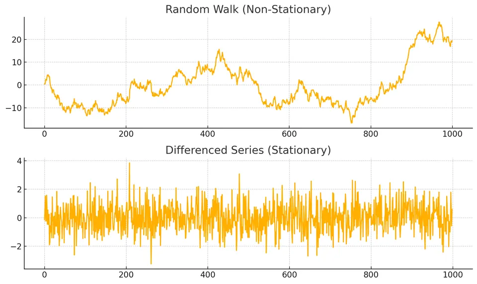
The upper panel shows the wandering random-walk level, while the lower panel shows the much more stable differenced series. The visual demonstrates why a difference-stationary process is modeled through its changes rather than by treating the original levels as stationary.
Formal Tests for Stationarity
Visual inspection can reveal trends, changing variance, or structural breaks, but formal tests provide additional evidence. The ADF and KPSS tests are useful together because their null hypotheses point in opposite directions.
Augmented Dickey–Fuller (ADF) Test
The ADF test evaluates a unit-root null using a regression of the form:
$$ \Delta X_t = \alpha + \beta t + \gamma X_{t-1} + \sum_{i=1}^{p} \delta_i \Delta X_{t-i} + \epsilon_t $$
where $\Delta X_t = X_t - X_{t-1}$ and $p$ lagged differences absorb serial correlation. The hypotheses are:
- $H_0$: $\gamma=0$, corresponding to a unit root under the chosen deterministic specification.
- $H_1$: $\gamma<0$, corresponding to stationarity around the included deterministic terms.
A sufficiently negative test statistic, or a small p-value, provides evidence against the unit-root null. The conclusion depends on whether the regression includes an intercept, a trend, or other deterministic terms.
KPSS Test
The Kwiatkowski–Phillips–Schmidt–Shin (KPSS) test reverses the direction of evidence:
- $H_0$: the series is level-stationary or trend-stationary, depending on the test specification;
- $H_1$: the stationarity assumption is violated.
Using both tests helps organize the evidence:
| ADF result | KPSS result | Interpretation |
|---|---|---|
| Reject unit-root null | Fail to reject stationarity | Evidence supports stationarity |
| Fail to reject unit-root null | Reject stationarity | Evidence supports non-stationarity |
| Reject | Reject | Possible break, deterministic misspecification, or other model mismatch; inspect the series |
| Fail to reject | Fail to reject | Evidence is inconclusive; power may be limited |
Student guide: stationarity is a modeling condition
Stationarity is not a synonym for “the plot looks flat.” It describes which features of the joint distribution remain unchanged when the time index is shifted. The version needed depends on the model and question.
Strict and weak stationarity
A process is strictly stationary if, for every collection of times and every shift $h$,
$$ (X_{t_1},\ldots,X_{t_k}) \overset{d}{=} (X_{t_1+h},\ldots,X_{t_k+h}). $$
Weak stationarity requires only:
$$ E(X_t)=\mu, \qquad \mathrm{Var}(X_t)=\gamma(0), \qquad \mathrm{Cov}(X_t,X_{t-h})=\gamma(h), $$
with no dependence on $t$. Many ARMA calculations use weak stationarity. Gaussian processes with constant mean and covariance are strictly stationary as well, but non-Gaussian weakly stationary processes need not be strictly stationary.
Numerical AR(1) example
Consider
$$ X_t=1+0.8X_{t-1}+\varepsilon_t, \qquad \mathrm{Var}(\varepsilon_t)=1. $$
The stationary mean is
$$ \mu=\frac{1}{1-0.8}=5, $$
and the stationary variance is
$$ \gamma(0)=\frac{1}{1-0.8^2}=2.7778. $$
The lag-1 covariance is
$$ \gamma(1)=0.8\gamma(0)=2.2222, $$
and the lag-1 correlation is $0.8$. The process can move substantially from one observation to the next while its distribution remains stable over time.
If $\phi=1$, the mean formula divides by zero and the variance does not settle. This is the unit-root boundary. If $|\phi|>1$, deviations grow and the process is explosive.
Deterministic trend versus stochastic trend
For
$$ y_t=10+0.2t+\varepsilon_t, $$
subtracting the deterministic trend can produce a stationary remainder. For a random walk,
$$ y_t=y_{t-1}+\varepsilon_t, $$
the uncertainty accumulates permanently. Both can look like an upward trend in one realization, but their forecasts and variance behavior differ.
Use domain knowledge, differencing behavior, plots, and diagnostics together. A stationarity test can assess a statistical specification, but it cannot identify the scientific mechanism by itself.
ADF and KPSS are complementary
The Augmented Dickey-Fuller test has a unit-root null. The KPSS test usually has a stationarity null. Their p-values are not interchangeable:
| ADF | KPSS | reading |
|---|---|---|
| reject unit root | fail to reject stationarity | evidence for stationarity |
| fail to reject unit root | reject stationarity | evidence against stationarity |
| both reject | possible trend stationarity, break, or misspecification | inspect plots and specifications |
| neither reject | low power or insufficient information | gather more evidence |
The outcome depends on whether a constant or trend is included, lag selection, sample length, and structural breaks. Tests should support a modeling decision rather than replace it.
Transformations
Common transformations have different meanings:
- log or Box-Cox: stabilize a variance that grows with level;
- detrending: remove a specified deterministic mean structure;
- first difference: model changes from one period to the next;
- seasonal difference: compare observations one seasonal cycle apart;
- seasonal adjustment: remove a repeating component before modeling residual dynamics.
After transforming, inspect the transformed series. The goal is not to erase every pattern; it is to create a series whose remaining structure is appropriate for the proposed model.
Local stationarity
Real data can be approximately stationary over a moving window and non-stationary globally. Examine rolling:
$$ \hat\mu_t=\frac1w\sum_{j=0}^{w-1}y_{t-j}, \qquad \hat\sigma_t^2=\frac1{w-1}\sum_{j=0}^{w-1}(y_{t-j}-\hat\mu_t)^2. $$
The window size $w$ is a resolution choice. A short window reacts quickly but is noisy; a long window smooths changes and can conceal a break.
Stationarity workflow
- Plot the level and relevant transforms.
- Inspect rolling moments and missingness.
- Check ACF behavior and seasonal lags.
- State the deterministic terms used in any test.
- Use ADF/KPSS or other tests as evidence, not as a single decision rule.
- Fit a simple candidate after transformation.
- Diagnose residuals and forecast behavior.
- Reassess whether the transformation matches the deployment question.