Confidence Intervals
A confidence interval (CI) is a range of plausible values for a population parameter, such as a mean or proportion, calculated from sample data. It supplements a point estimate by showing the uncertainty around that estimate.
Definition and Components
Many common confidence intervals can be written as:
$$ (\text{Point Estimate} - \text{Margin of Error}, \ \text{Point Estimate} + \text{Margin of Error}) $$
where:
- The point estimate is a single estimate of the population parameter based on the sample, such as a sample mean or sample proportion.
- The margin of error measures the uncertainty around the point estimate.
The margin of error is often:
$$ \text{Margin of Error} = \text{Critical Value} \times \text{Standard Error} $$
The confidence level, commonly 90%, 95%, or 99%, describes the long-run coverage rate of the interval-construction method. Holding everything else fixed, a higher confidence level produces a wider interval: coverage increases, but precision decreases.
A confidence interval is not limited to one particular probability distribution. Confidence intervals can be constructed for many different population parameters and data-generating distributions.
What changes is the method used to build the interval.
For example:
- For a population mean with known standard deviation, we often use the normal distribution.
- For a mean with unknown standard deviation, we commonly use the t-distribution.
- For proportions, we may use a normal approximation, Wilson interval, or exact binomial method.
- For variances, intervals often use the chi-square distribution.
- For ratios of variances, the F-distribution may be used.
- When the underlying distribution is unknown or complicated, bootstrap confidence intervals can be used.
The key requirement is that we know, estimate, or approximate the sampling distribution of the estimator.
For many common intervals, the general form is:
$$ \text{Estimate} \pm \text{Critical Value} \times \text{Standard Error} $$
but the critical value and standard error depend on the situation.
Confidence intervals can also be:
- Parametric, where a distributional model is assumed.
- Nonparametric, with fewer assumptions about the population distribution.
- Approximate, often relying on large-sample results such as the Central Limit Theorem.
- Exact, when the interval has the stated coverage under the assumed model.
Therefore, confidence intervals are broadly applicable, but not every confidence-interval formula works in every setting. The method must match the parameter, sample size, data type, and assumptions.
Example: Confidence Interval for the Mean
Suppose we simulate sample data from a population with a true mean of 50 and a standard deviation of 5. From the sample, we calculate the sample mean and construct a confidence interval around it.
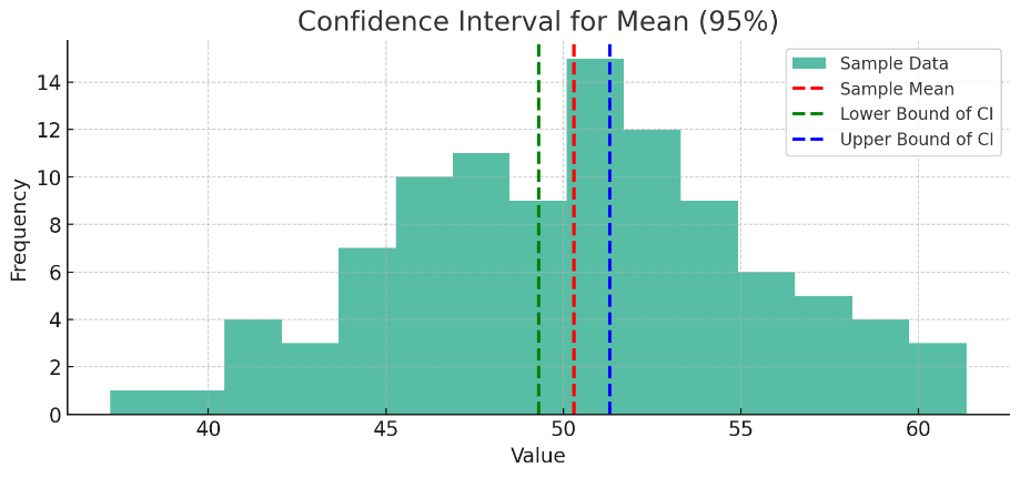
In the plot:
- The red dashed line represents the sample mean, which is the point estimate of the population mean.
- The green and blue dashed lines represent the lower and upper bounds of the 95% confidence interval.
A single interval either contains the true population mean or it does not. The 95% confidence level refers to the method: over many repeated samples, approximately 95% of intervals constructed in this way would contain the true mean.
Example: Confidence Intervals for Simulated Stock Returns
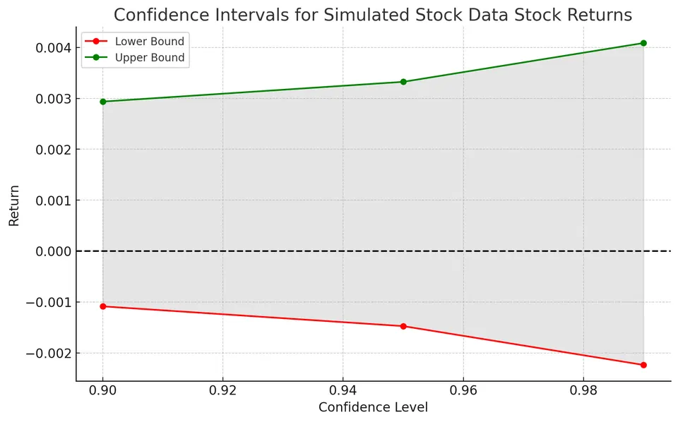
The plot shows confidence intervals for the mean of 252 synthetic (seeded, simulated) daily returns at 90%, 95%, and 99% confidence levels. The accompanying script generates the returns itself and does not download market data.
- The lower bound decreases as the confidence level increases.
- The upper bound increases as the confidence level increases.
- The shaded area represents the width of the confidence interval and expands at higher confidence levels.
- The horizontal line at zero shows whether an interval includes both positive and negative returns.
The 90% interval is narrower and therefore more precise, but its long-run coverage is lower. The 99% interval is wider, providing higher coverage at the cost of precision.
Constructing a Confidence Interval
Suppose the true approval rate among 150 million likely voters is 62%, and a poll surveys 1,200 voters to estimate that rate. Because the poll uses a sample rather than the full population, the estimate is subject to sampling variability. The standard error (SE) quantifies that variability.
In practice, the true approval rate is unknown. Here, the known value is used only to illustrate the sampling behavior of the estimator.
Step 1: Use the Central Limit Theorem
For a sufficiently large random sample, the sampling distribution of a sample proportion is approximately normal. If the population proportion is $p$, its theoretical standard error is:
$$ SE = \sqrt{\frac{p(1-p)}{n}} $$
where:
- $p = 0.62$ is the population proportion.
- $n = 1{,}200$ is the sample size.
Substituting the values:
$$ SE = \sqrt{\frac{0.62 \times 0.38}{1{,}200}} = \sqrt{0.0001963} \approx 0.014 $$
Thus, the standard error is approximately 0.014, or 1.4 percentage points.
In practice, the population proportion $p$ is unknown, so it is usually replaced by the observed sample proportion $\hat{p}$ when estimating the standard error.
Step 2: Construct the 95% Confidence Interval
A 95% confidence interval uses the critical value $z^* = 1.96$. The common approximation of two standard errors is close, but 1.96 is more precise.
Suppose the poll reports a sample proportion of 60%. The estimated standard error is:
$$ SE = \sqrt{\frac{0.60(0.40)}{1{,}200}} \approx 0.0141 $$
The confidence interval is:
$$ \text{Confidence Interval} = \hat{p} \pm z^* \times SE $$
where:
- $\hat{p} = 0.60$ is the sample proportion.
- $z^* = 1.96$ is the 95% critical value.
- $SE \approx 0.0141$.
Therefore:
$$ 0.60 \pm 1.96(0.0141) \approx 0.60 \pm 0.0277 $$
or approximately:
$$ 57.2\% \text{ to } 62.8\% $$
Using the rough critical value of 2 gives a very similar result.
Step 3: Understand Confidence vs. Probability
The population parameter is fixed, while the confidence interval varies from sample to sample. Therefore:
- A particular interval either contains the true population parameter or it does not.
- A 95% confidence procedure produces intervals that contain the true parameter in approximately 95% of repeated samples, assuming the method's conditions hold.
- In the frequentist framework, it is not strictly correct to say that there is a 95% probability that the fixed parameter lies inside one already-calculated interval.
Confidence Levels and Critical Values
Common confidence levels and their approximate standard-normal critical values are:
| Confidence level | Critical value $z^*$ |
|---|---|
| 90% | 1.645 |
| 95% | 1.960 |
| 99% | 2.576 |
A confidence interval based on a normal approximation is:
$$ \text{Estimate} \pm z^* \times SE $$
where the estimate is a sample statistic and $SE$ is its standard error.
For a confidence interval for a mean, the $t$-distribution is used instead of the standard normal distribution when the population standard deviation is unknown and estimated by $s$:
$$ \bar{x} \pm t^*_{n-1}\,\frac{s}{\sqrt{n}} $$
where $t^*_{n-1}$ is the critical value with $n-1$ degrees of freedom. It is larger than $z^*$ (for example, $t^*_{29}=2.045$ at 95% confidence versus $z^*=1.960$) and approaches $z^*$ as $n$ grows. This interval is exact when the data are normal and approximate otherwise.
Estimating the Standard Error
When an unknown population quantity appears in the standard-error formula, it is often replaced by a sample estimate. This is called a plug-in estimate. For example, $\hat{p}$ can replace an unknown population proportion $p$, and the sample standard deviation $s$ can replace an unknown population standard deviation $\sigma$.
A bootstrap estimate is different: it repeatedly resamples the observed data with replacement and uses the variability of the resulting estimates to approximate the standard error.
For a sample proportion of 60% from a sample of 1,000 people:
$$ SE = \sqrt{\frac{\hat{p}(1-\hat{p})}{n}} $$
where:
- $\hat{p} = 0.60$.
- $n = 1{,}000$.
Substituting the values:
$$ SE = \sqrt{\frac{0.60 \times 0.40}{1{,}000}} = \sqrt{0.00024} \approx 0.0155 $$
The estimated standard error is therefore about 1.55 percentage points.
Constructing the Confidence Interval
Using a 95% confidence level with $z^* = 1.96$:
$$ \text{Confidence Interval} = 0.60 \pm 1.96(0.0155) $$
$$ \text{Confidence Interval} = 0.60 \pm 0.0304 = (0.5696,\ 0.6304) $$
Expressed as percentages, the interval is approximately 56.96% to 63.04%.
Width of a Confidence Interval
The width of a confidence interval is determined by its margin of error:
$$ \text{Margin of Error} = z^* \times SE $$
Two factors have an especially important effect:
- A larger sample size reduces the standard error and narrows the interval. Because standard error is generally proportional to $1/\sqrt{n}$, halving the interval width requires approximately four times the sample size, all else being equal.
- A lower confidence level, such as 90% instead of 95%, uses a smaller critical value and produces a narrower interval, but also lowers the long-run coverage rate.
Interpreting the Confidence Level
The confidence level is the proportion of intervals that would contain the true parameter over repeated applications of the same sampling and interval-construction procedure.
For example, if we repeatedly took random samples and calculated a 95% confidence interval from each one, approximately 95% of those intervals would contain the true population parameter, provided the assumptions behind the method were satisfied.
Example: Health-App Step Counts
Consider two health apps that estimate average daily steps:
- App X reports a point estimate of 10,300 steps per day.
- App Y reports a 90% confidence interval of $10{,}000 \pm 500$ steps per day, or 9,500 to 10,500 steps per day.
App Y communicates both the estimate and its uncertainty. This makes the result more informative, assuming the sample and data-collection methods are reliable.
A 95% Confidence Interval for a Parameter
When the sampling distribution of a point estimate is approximately normal, a 95% confidence interval can be written as:
$$ \text{Point Estimate} \pm 1.96 \times SE $$
The value 1.96 comes from the standard normal distribution: approximately 95% of its probability lies between $-1.96$ and $1.96$.
Example: Carry-on Baggage Weight
Suppose the mean weight in a sample of carry-on bags is 3.2 kg, with a standard error of 0.053 kg. Assuming the normal approximation is appropriate, the 95% confidence interval is:
$$ \text{Confidence Interval} = \text{Sample Mean} \pm (\text{Critical Value} \times \text{Standard Error}) $$
$$ 3.2 \pm 1.96(0.053) = 3.2 \pm 0.10388 = (3.09612,\ 3.30388) $$
Thus, the estimated population mean weight is between approximately 3.096 kg and 3.304 kg at the 95% confidence level.
Example: Calibrating a Digital Thermometer
Suppose a digital thermometer is tested repeatedly at a known reference temperature. A confidence interval can be used to estimate the thermometer's mean reading at that reference temperature. It does not, by itself, describe the accuracy of every individual future reading.
A 95% confidence interval for the mean reading has the form:
$$ CI = \bar{x} \pm \text{Critical Value} \times SE $$
where $\bar{x}$ is the sample mean reading and $SE$ is the standard error of the sample mean. If the population standard deviation $\sigma$ were known, $SE=\sigma/\sqrt{n}$ and the critical value would be $z^*$. Here $\sigma$ is unknown, so we use $SE=s/\sqrt{n}$ and a $t$ critical value.
Suppose 30 trials produce a mean reading of 37.0°C and a sample standard deviation of 0.5°C:
$$ SE = \frac{0.5}{\sqrt{30}} \approx 0.0913 $$
With $df=29$, $t^*=2.045$, so:
$$ CI = 37.0 \pm 2.045(0.0913) \approx 37.0 \pm 0.187 = (36.81,\ 37.19) $$
Using the normal critical value $1.96$ instead would give the slightly narrower interval $37.0 \pm 0.179$, which understates the uncertainty a little for $n=30$.
This interval estimates the thermometer's mean reading under the test conditions.
Common Misconceptions
A common mistake is to interpret a 95% confidence interval as meaning, “There is a 95% chance that the true mean lies within this specific interval.”
Under the frequentist interpretation, the population parameter is fixed and the interval is random before the data are observed.
The correct interpretation is that the method used to construct the interval captures the true population parameter in approximately 95% of repeated samples, assuming its conditions are met.
Changing the Confidence Level
For a normally distributed point estimate with known standard error:
$$ \text{Point Estimate} \pm z^* \times SE $$
Here, $z^*$ is the critical value for the selected confidence level, and $z^* \times SE$ is the margin of error.
Example: Blood-Pressure Readings
Suppose blood-pressure readings are normally distributed, the population standard deviation is 12 mmHg, and a random sample of 50 patients has a mean of 130 mmHg. We can calculate 90% and 99% confidence intervals for the population mean.
Step 1: Calculate the Standard Error
$$ SE = \frac{\sigma}{\sqrt{n}} = \frac{12}{\sqrt{50}} \approx 1.697 $$
Step 2: Determine the Critical Values
- For a 90% confidence level, $z^* \approx 1.645$.
- For a 99% confidence level, $z^* \approx 2.576$.
Step 3: Calculate the Confidence Intervals
For 90% confidence:
$$ 130 \pm 1.645(1.697) = 130 \pm 2.79 = (127.21,\ 132.79) $$
For 99% confidence:
$$ 130 \pm 2.576(1.697) = 130 \pm 4.37 = (125.63,\ 134.37) $$
The 99% confidence interval is wider than the 90% confidence interval. This illustrates the trade-off between higher confidence and greater precision.
Prediction Intervals vs. Confidence Intervals
A confidence interval estimates a population parameter, such as the population mean. A prediction interval gives a range of plausible values for a single future observation.
A prediction interval is wider because it must account for both:
- Uncertainty in the estimated mean.
- Natural variation among individual observations.
For a normally distributed population with known $\sigma$, a 95% prediction interval for a new observation $X_{\text{new}}$ is:
$$ \bar{x} \pm z_{1-\alpha/2}\sigma\sqrt{1+\frac{1}{n}} $$
When $\sigma$ is unknown and estimated by the sample standard deviation $s$, the $t$-distribution is used:
$$ \bar{x} \pm t_{1-\alpha/2,\,n-1} s\sqrt{1+\frac{1}{n}} $$
| Aspect | Confidence interval | Prediction interval |
|---|---|---|
| Target | Population parameter, such as $\mu$ | One future observation |
| Width | Narrower | Wider |
| Effect of increasing $n$ | Typically shrinks toward zero | Approaches a nonzero width determined by the underlying variability |
This distinction is especially important in regression. At a given value of $x$, a confidence interval for the mean response is narrower than a prediction interval for one new response.