Autoregressive (AR) Models in Time Series Analysis

An autoregressive model predicts the next observation from observed values of the same series. If high demand tends to be followed by high demand, lagged demand contains predictive information. An AR equation assigns coefficients to that information and adds a new shock for the part the past did not predict.

The model is more than a regression with convenient predictors. Its output becomes a predictor at the next date, so a shock can feed through the recursion many times. The coefficients jointly determine whether that feedback fades, alternates, oscillates, or grows.

Three questions must be kept separate. Order asks which observed lags enter directly. Stability asks what repeated application of those coefficients does to a deviation. Forecast uncertainty asks how unknown future shocks combine over the prediction horizon. The ACF, PACF, root calculations, and forecast formulas below describe different consequences of the same recursion.

Worked calculation: one AR(2) update

Take

$$ X_t=0.4+0.6X_{t-1}-0.2X_{t-2}+\varepsilon_t. $$

If $X_{t-1}=3$, $X_{t-2}=2$, and the new shock is $\varepsilon_t=0.5$, then

$$ X_t=0.4+0.6(3)-0.2(2)+0.5=2.3. $$

Before the new shock is observed, the conditional mean is

$$ E(X_t\mid X_{t-1}=3,X_{t-2}=2)=1.8. $$

The predictable part is $0.4+0.6(3)-0.2(2)=1.8$. The innovation of 0.5 raises the realized value to 2.3. At the next date, that higher observation becomes one of the lagged predictors, so the shock can influence later values as well. The AR polynomial $1-0.6B+0.2B^2$ records the feedback coefficients; its roots determine whether those subsequent effects decay.

From observed lags to a conditional prediction

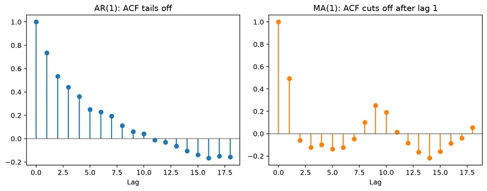
Autoregressive (AR) models describe serial dependence by expressing the current value of a time series as a linear function of its own past values plus a new innovation. The order $p$ in AR($p$) specifies how many lags appear directly in the model.

Definition of Autoregressive Models

An autoregressive model of order $p$, AR($p$), is

$$ X_t=c+\phi_1X_{t-1}+\phi_2X_{t-2}+\dots+\phi_pX_{t-p}+\varepsilon_t, $$

or equivalently,

$$ X_t=c+\sum_{i=1}^{p}\phi_iX_{t-i}+\varepsilon_t. $$

Each coefficient describes a contribution with the other included lags held fixed. In AR(2), $\phi_1$ controls the contribution of the previous observation and $\phi_2$ the contribution of the observation before it. Their combined dynamic effect can differ markedly from either coefficient considered alone. Interpreting a positive coefficient as “persistent growth” without checking the full recursion can therefore be misleading.

Components of the AR($p$) Model

• $X_t$ is the value of the series at time $t$.
• $c$ is the intercept. For a stationary AR process, it is generally not equal to the unconditional mean.
• $\phi_i$ is the coefficient on lag $i$.
• $X_{t-i}$ is the observation $i$ periods before time $t$.
• $\varepsilon_t$ is the innovation, usually modeled as white noise with mean zero and constant variance.

Under a weak white-noise assumption,

$$ E(\varepsilon_t)=0, \qquad \mathrm{Var}(\varepsilon_t)=\sigma^2, $$

and innovations are uncorrelated across time. Some estimation and forecasting results use the stronger assumption that the innovations are independent, often Gaussian.

When the innovation has zero conditional mean given the past, the lagged part is the one-step conditional-mean forecast. With only weak-white-noise assumptions, the same equation can describe linear prediction relationships without ruling out nonlinear predictability. State the stronger assumption when interpreting the fitted equation as the complete conditional mean rather than only a linear dynamic model.

Order of an AR Model

The order $p$ is the largest lag included in the AR polynomial. In the usual consecutive-lag specification, it gives the number of lagged observations entered as predictors. An intermediate coefficient may be zero, so the order need not equal the number of nonzero coefficients.

An AR(1) uses one lag:

$$ X_t=c+\phi_1X_{t-1}+\varepsilon_t. $$

An AR(2) uses two lags:

$$ X_t=c+\phi_1X_{t-1}+\phi_2X_{t-2}+\varepsilon_t. $$

More generally, an AR($k$) is

$$ X_t=c+\sum_{i=1}^{k}\phi_iX_{t-i}+\varepsilon_t. $$

Adding a lag lets the next prediction depend directly on an older observation. It also adds a coefficient estimated from a finite, dependent record and removes another starting row from the lagged design matrix. Several adjacent lag columns can be strongly correlated. An apparently improved training fit may therefore come with more variable coefficients and worse later forecasts.

Example: AR(2) Model in Practice

Suppose the current measurement $y_t$ is modeled using the previous two measurements:

$$ y_t=B_0+B_1y_{t-1}+B_2y_{t-2}+w_t. $$

Here $B_0$ is the intercept, $B_1$ and $B_2$ are the lag coefficients, and $w_t$ is the innovation. Conditional on the two observed lags, the model's one-step mean forecast is

$$ E(y_t\mid y_{t-1},y_{t-2})=B_0+B_1y_{t-1}+B_2y_{t-2}. $$

The innovation $w_t$ is the observed value minus that conditional mean. Before the observation arrives, the forecast sets the expected innovation to zero; afterward, the realized innovation measures the part of the update that the two lagged values did not predict.

General Interpretation of AR($p$) Models

An AR($p$) model resembles a regression whose predictors are lagged values of the response itself:

$$ X_t=c+\phi_1X_{t-1}+\dots+\phi_pX_{t-p}+\varepsilon_t. $$

The regression representation explains how to estimate a one-step equation from observed lagged rows. The recursion explains what happens after that equation is iterated. A coefficient estimate that fits the available rows well can still produce explosive multi-step forecasts. Evaluate the fitted polynomial as well as the regression residuals before using the equation beyond the observed sample.

Estimation of Parameters

Several methods are commonly used to estimate $c$ and the AR coefficients.

Least squares estimation constructs one row for each date with all required lags available and minimizes squared one-step residuals. For AR(2), that row contains an intercept, $X_{t-1}$, and $X_{t-2}$; the target is $X_t$. The first two observations provide predictors but cannot supply complete target rows. The estimator is simple because these predictors are observed, unlike the latent shock lags in an MA model.

Yule-Walker estimation starts from covariance relationships rather than individual prediction rows. A stationary AR process forces its autocovariances to satisfy linear equations involving the AR coefficients. Replacing those covariances with sample estimates gives a system to solve. This method makes the stationarity assumption explicit and provides a useful independent view of the fitted dependence pattern.

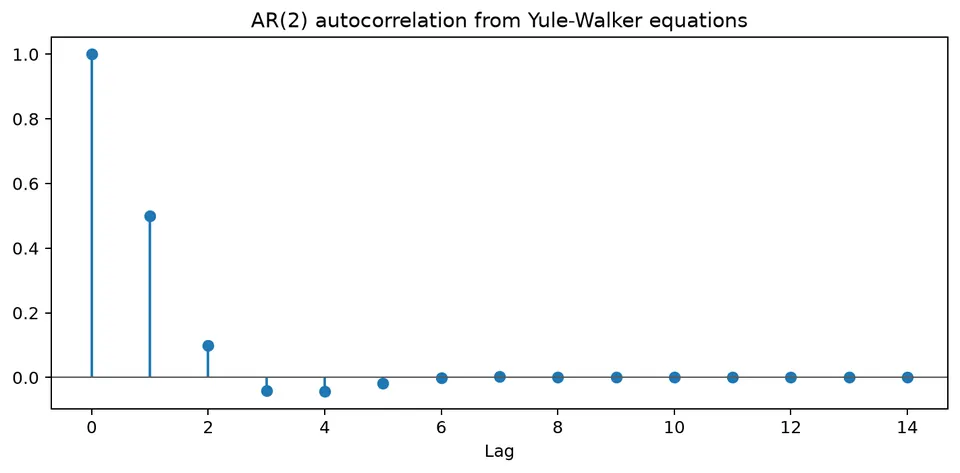
The recursion makes that moment relationship concrete: once the AR coefficients are fixed, the autocorrelations satisfy a corresponding lag recursion. Yule-Walker estimation reverses this relationship, using sample autocovariances to estimate the AR coefficients.

Maximum likelihood estimation specifies the probability distribution of the observations under the model and chooses parameters that make the observed path most likely. In a Gaussian model this uses both prediction errors and their variances, with a specified treatment of the initial observations. Exact and conditional likelihoods can therefore differ in short samples even when they share the same AR equation.

Different implementations can handle initialization and finite samples differently, so estimates need not be identical even when they target the same AR specification.

Model Selection for Autoregressive (AR) Models

Choosing $p$ requires balancing fit against complexity. ACF and PACF patterns can suggest plausible orders, while information criteria and out-of-sample evaluation help distinguish among candidate models.

Autocorrelation Function (ACF)

The sample autocorrelation at lag $k$ can be written as

$$ r_k= \frac{\sum_{i=1}^{n-k}(Y_i-\bar Y)(Y_{i+k}-\bar Y)} {\sum_{i=1}^{n}(Y_i-\bar Y)^2}. $$

For a stationary AR($p$), the population ACF usually tails off rather than becoming exactly zero after lag $p$. Depending on the coefficients, the decay can be monotone, alternating, or damped and oscillatory.

For example, a stationary AR(1) with $\phi=0.8$ has population autocorrelation $\rho_k=0.8^k$.

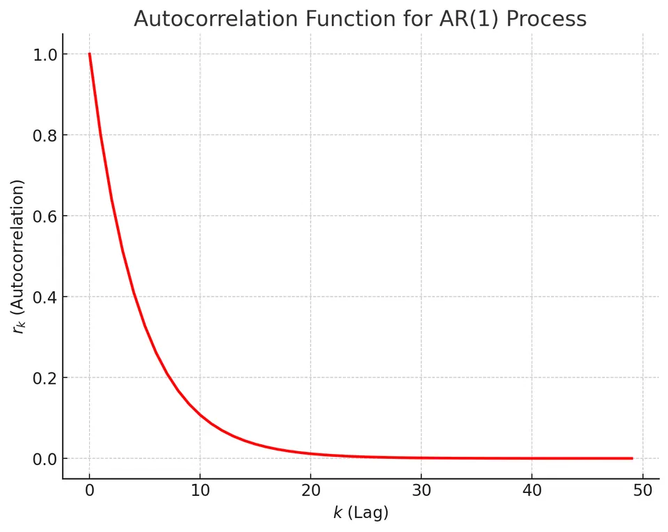
The gradual decay in this plot is the kind of pattern that suggests autoregressive persistence, although a sample ACF alone does not identify the order uniquely.

Partial Autocorrelation Function (PACF)

The partial autocorrelation function (PACF) measures the remaining linear association between $Y_t$ and $Y_{t-k}$ after projecting out the intermediate lags $1,\ldots,k-1$. This linear adjustment is the relevant operation; it does not generally imply conditional independence or establish a direct causal effect.

After the first $p$ lags are included, an older lag adds no further linear predictive information in a correctly specified causal AR($p$). That produces the population PACF cutoff. It does not say that an older observation is uncorrelated with the current observation: its influence can travel through the intermediate lags, which is why the ordinary ACF can remain nonzero well beyond $p$.

The following plots illustrate the typical ACF and PACF behavior of an AR(2):

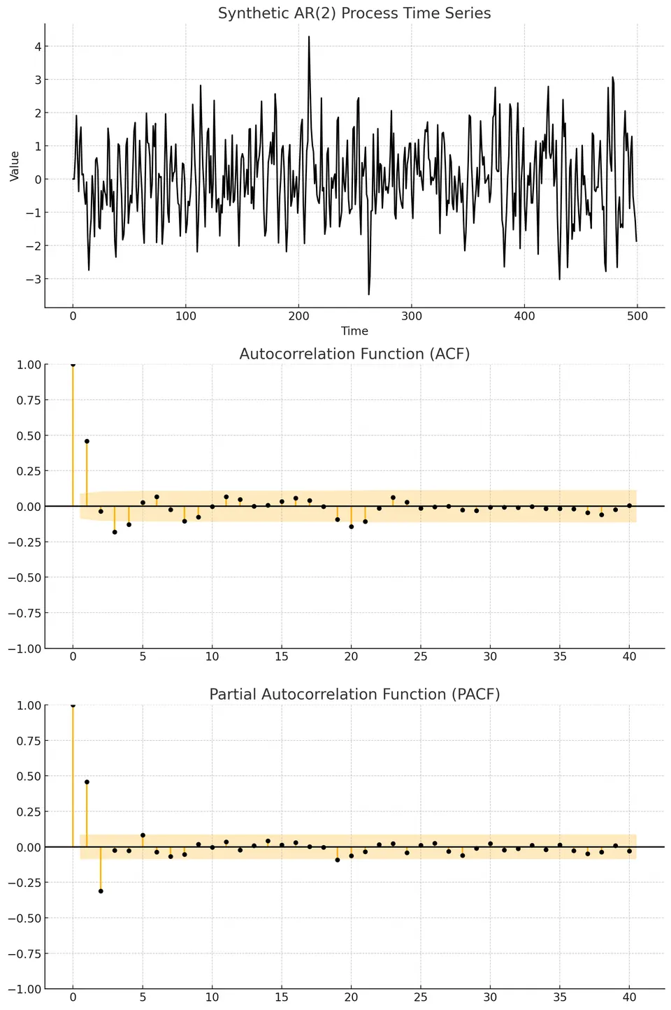
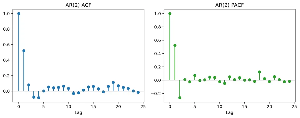
The key pattern is that the ACF tails off while the PACF concentrates its population signal in the first two lags. These are identification heuristics, not a substitute for fitting and checking candidate models.

Information Criteria for Model Selection

Information criteria compare likelihood fit with a penalty for additional parameters.

Akaike Information Criterion (AIC)

The AIC is

$$ \mathrm{AIC}=-2\ln(L)+2k, $$

where $L$ is the maximized likelihood and $k$ is the number of estimated parameters counted under the chosen convention. Lower values are preferred when comparing models fitted to the same response data with the same likelihood basis.

Bayesian Information Criterion (BIC)

The BIC is

$$ \mathrm{BIC}=-2\ln(L)+k\ln(n), $$

where $n$ is the sample size. Because its penalty grows with $n$, BIC generally penalizes additional parameters more strongly than AIC in larger samples.

Neither criterion establishes that a model is adequate. Residual diagnostics and forecast evaluation are still required.

Steps for Selecting the Optimal AR Model Order

A practical selection process is:

1. inspect the transformed series, ACF, and PACF to propose a small set of candidate orders;
2. fit those AR models using a consistent estimation method and sample;
3. compare AIC or BIC within that candidate set;
4. inspect residual autocorrelation and parameter stability;
5. compare temporal forecast performance when forecasting is the goal.

For example, suppose candidate models give

AR(2) has the smallest criterion values within this particular candidate set. The comparison says that its improvement in likelihood outweighs the chosen parameter penalty relative to these alternatives. It does not test whether the candidates handled trend, seasonality, or breaks correctly. Check those features, residual dependence, and chronological forecast performance before treating the selected order as adequate.

Properties of AR Models

Stationarity in AR models

For the standard causal AR($p$) model, the roots of

$$ 1-\phi_1z-\cdots-\phi_pz^p=0 $$

must lie outside the unit circle. For AR(1), this reduces to $|\phi_1|<1$. At $\phi_1=\pm1$, the usual finite-variance stationary solution breaks down.

If $|\phi_1|>1$, a bilateral stationary solution can be written only in a noncausal form that depends on future shocks. That mathematical possibility is different from the standard causal AR model used for forecasting, where current values are generated from past information.

Autocorrelation Function (ACF)

For a stationary causal AR model, the ACF tails off with lag. The exact pattern can be exponential, alternating, or damped and oscillatory, depending on the roots of the AR recursion.

Partial Autocorrelation Function (PACF)

For an ideal population AR($p$), the PACF cuts off after lag $p$. This is why the PACF is useful for proposing AR orders, especially when the series is stationary and the sample is reasonably long.

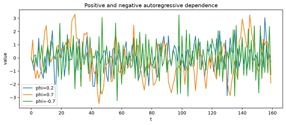
The persistence figure shows how coefficients closer to the unit-root boundary make shocks decay more slowly. That same persistence appears as a slower ACF decay and slower mean reversion in forecasts.

Example: AR(2) Model in Time Series Forecasting

Consider

$$ X_t=c+\phi_1X_{t-1}+\phi_2X_{t-2}+\varepsilon_t. $$

Suppose

• $c=3$,
• $\phi_1=0.6$,
• $\phi_2=-0.2$,
• $X_{t-1}=10$,
• $X_{t-2}=5$.

AR(2) Model Equation

Substituting the observed lags gives

$$ X_t=3+0.6(10)-0.2(5)+\varepsilon_t =8+\varepsilon_t. $$

Calculation

The one-step conditional mean is therefore

$$ \hat X_{t\mid t-1}=8. $$

The realized observation differs from 8 by the new innovation $\varepsilon_t$.

Interpretation

The calculation gives a mean forecast of 8 for this particular pair of observed lags. A new innovation can put the realized observation above or below 8. For a second step ahead, the model uses the first forecast in place of the future observation that is not yet known; it still uses the last actual observation for the older lag. This replacement is the essential difference between evaluating one fitted row and issuing a multi-step forecast.

Visualization

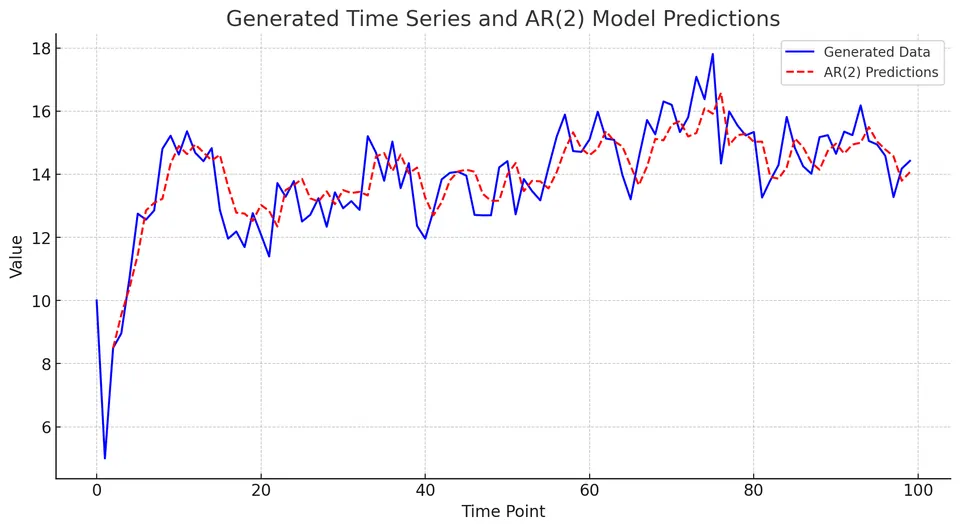
The blue line shows a simulated AR(2) series and the red dashed line shows fitted or predicted values. The relevant comparison is how well the AR(2) conditional mean follows the serial dependence in the data; the remaining deviations should behave like innovations rather than a systematic pattern.

Limitations of AR Models

Linearity assumption. AR models describe linear dependence on past values. Nonlinear thresholds, asymmetric responses, and other nonlinear dynamics require a different specification.

Stationarity requirement. The standard AR theory in this chapter assumes a stationary causal process. Trends, seasonality, unit roots, or structural breaks should be modeled or transformed rather than absorbed by an arbitrarily high AR order.

Sensitivity in parameter estimation. Outliers, near-unit roots, collinear lag columns, and model misspecification can make coefficient estimates unstable or misleading.

Complexity in model selection. ACF/PACF patterns and information criteria narrow the candidate set but do not determine the correct model automatically, especially in short or structurally changing series.

Risk of overfitting. Increasing $p$ can improve in-sample fit while degrading forecast performance. Temporal validation and parsimonious specifications are therefore important.

How feedback determines means, roots, and forecasts

An AR model explains the current value using observed past values:

$$ y_t=c+\phi_1y_{t-1}+\cdots+\phi_py_{t-p}+\varepsilon_t. $$

The observed lags act as regressors, but stationarity and persistence are determined by the AR polynomial rather than by the regression interpretation alone.

AR(1) numbers

For

$$ y_t=1+0.8y_{t-1}+\varepsilon_t, \qquad \mathrm{Var}(\varepsilon_t)=1, $$

the stationary mean is $5$ and the variance is

$$ \frac{1}{1-0.8^2}=2.7778. $$

If the latest centered value is $y_T-\mu=2$, the one-step conditional mean deviation is

$$ \hat y_{T+1|T}-\mu=0.8(2)=1.6, $$

and the five-step deviation is

$$ \hat y_{T+5|T}-\mu=0.8^5(2)=0.6554. $$

The centered deviation is multiplied by 0.8 each step. A deviation of 2 becomes 1.6 after one forecast step and about 0.655 after five; the forecast moves back toward the mean 5 rather than continuing a straight line from the latest observation. Taking expectations of the AR equation gives $\mu=c+\phi\mu$, which explains why the intercept 1 produces a stationary mean of 5 instead of 1.

AR(2) roots

For

$$ y_t=0.6y_{t-1}-0.2y_{t-2}+\varepsilon_t, $$

the homogeneous recursion has characteristic equation

$$ r^2-0.6r+0.2=0. $$

Its discriminant is $0.36-0.8=-0.44$, so

$$ r=\frac{0.6\pm i\sqrt{0.44}}{2}. $$

The roots have modulus $\sqrt{0.2}\approx0.447$, below 1, so the impulse response oscillates while decaying. These recursion roots are the reciprocals of the roots of the AR polynomial written in the backshift variable; the two common root conventions therefore use opposite inside/outside unit-circle statements.

Complex roots can produce alternating or cyclical ACF patterns without implying deterministic seasonality.

Estimation and intercepts

For AR($p$), create a design matrix from rows $t=p+1,\ldots,T$:

$$ \mathbf y= \begin{bmatrix} y_{p+1}\\ \vdots\\ y_T \end{bmatrix}, \qquad \mathbf X= \begin{bmatrix} 1&y_p&\cdots&y_1\\ \vdots&\vdots&&\vdots\\ 1&y_{T-1}&\cdots&y_{T-p} \end{bmatrix}. $$

When $X^\top X$ is nonsingular, the conditional least-squares estimate is

$$ \hat\beta=(X^\top X)^{-1}X^\top y. $$

A deterministic trend, seasonal terms, or highly collinear lag columns can make this calculation unstable. Conditional and exact likelihood methods can handle initial observations and innovation variance differently, so their finite-sample estimates need not coincide with conditional least squares. The displayed matrix inverse is an algebraic expression; numerical implementations should solve the least-squares problem directly rather than explicitly form the inverse.

The intercept $c$ is not the stationary mean. For AR(1),

$$ \mu=\frac{c}{1-\phi}. $$

For stationary AR($p$),

$$ \mu=\frac{c}{1-\sum_{j=1}^{p}\phi_j}, $$

provided the denominator is nonzero.

Forecast uncertainty

For a centered AR(1),

$$ \hat y_{T+h\mid T}=\phi^hy_T, $$

and the $h$-step forecast-error variance is

$$ \mathrm{Var}(e_{T+h}) =\sigma^2\sum_{j=0}^{h-1}\phi^{2j}. $$

A future shock at the last forecast date enters with coefficient 1, the preceding future shock with coefficient $\phi$, and earlier future shocks with higher powers of $\phi$. Squaring those weights and adding their variance contributions gives the forecast-error variance above. As the horizon grows, increasingly many shocks remain unknown, but their decaying weights keep the total below a finite limit in the stationary model.

Overfitting and stability

Increasing $p$ can reduce in-sample error while making coefficient estimates and forecasts unstable. Check root location, coefficient uncertainty, residual autocorrelation, parameter stability over time, and temporal forecast performance.

A model can be technically stationary yet practically very persistent when a root lies close to the unit-circle boundary. In that case, finite-sample estimates and long-horizon forecast intervals deserve extra scrutiny.

Formula reference