Stochastic Processes and White Noise

Imagine observing daily demand over the same month under many possible sequences of customer arrivals. Each possible sequence is a path. At a fixed date, the different possible demands form a random variable. A stochastic process specifies how those random variables fit together across dates, including their dependence.

The dataset in hand is one path, not the collection of every possible path. A time-series model uses that observed sequence to describe other values the process could have produced and uncertainty about values still to come. This distinction is essential when interpreting a wandering path, a rolling variance, or a model forecast.

White noise is the simplest second-order reference for shocks: a zero mean, a common finite variance, and zero covariance across different dates. Those conditions make linear correlation with past shocks vanish. They do not by themselves make the shocks independent or rule out predictability in their magnitudes. Forecast models need to state whether they assume only these moment conditions or a stronger conditional-mean or distributional property.

Worked calculation: shocks versus accumulated shocks

Let $\varepsilon_t$ be independent with mean 0 and variance 1. It is white noise because

$$ \mathrm{Cov}(\varepsilon_t,\varepsilon_{t-h})=0\quad(h\ne0). $$

Now define a random walk by $X_t=X_{t-1}+\varepsilon_t$ with fixed $X_0$. After 100 steps,

$$ X_{100}=X_0+\sum_{j=1}^{100}\varepsilon_j, \qquad \mathrm{Var}(X_{100})=100. $$

A new increment adds another independent variance contribution of 1. After 100 increments the level therefore has variance 100, even though the variance of each individual increment is still 1. A typical path can move up or down for an extended period without a deterministic trend in its mean. The nonstationarity is established by the variance calculation, not by deciding whether one plotted path looks like it is trending.

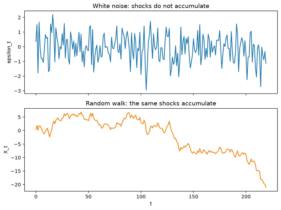
The figure contrasts the stable spread of the shocks with the increasing dispersion of their cumulative sum. The visual distinction mirrors the variance calculation above.

Processes, random variables, and observed paths

A time series is one observed path from an underlying stochastic process: a family of random variables indexed by time,

$$ \{X_t:t\in T\}. $$

Fixing $t$ asks about the distribution of a quantity at one date. Fixing a realization instead gives the sequence $x_1,\ldots,x_n$ observed through time. A histogram pools values from that path and hides their order. It cannot show whether large values cluster, whether a level shift occurred, or whether one observation helps predict the next. Those are properties of the joint time-indexed process.

Innovations

To forecast, separate the part that can be predicted from the part that arrives as new information. The decomposition below expresses that idea, but it becomes mathematically meaningful only after specifying the information used by $m_t$ and the type of prediction it represents:

$$ X_t=m_t+\varepsilon_t. $$

When $m_t=E(X_t\mid\mathcal F_{t-1})$, the predictable term is the conditional mean given the available past, and $\varepsilon_t$ is a conditional-mean innovation. In a linear prediction model, an innovation can instead mean the error of the best linear predictor. That error is orthogonal to past linear predictors; a zero conditional mean requires an additional assumption, such as joint Gaussianity or an explicit conditional-mean model.

For a conditional-mean innovation, any function of the available past has zero expected product with the innovation, subject to the required integrability. If a past pattern could systematically predict its mean, that pattern should already be included in $m_t$. A linear innovation makes a narrower promise: no remaining linear combination of the chosen past variables improves the prediction. Neither promise implies a constant conditional variance.

White Noise

A weak white-noise process $\{\varepsilon_t\}$ satisfies

$$ E[\varepsilon_t]=0, \qquad \mathrm{Var}(\varepsilon_t)=\sigma^2, \qquad \mathrm{Cov}(\varepsilon_t,\varepsilon_{t-h})=0\quad(h\ne0). $$

The three conditions play separate roles. Zero mean locates the shocks around zero. Constant finite variance supplies one common scale. Zero nonzero-lag covariance removes linear serial association. Adding independence rules out all cross-time dependence; adding a jointly Gaussian distribution makes covariance sufficient to describe the dependence. Merely giving each marginal shock a normal distribution is not the same as specifying a jointly Gaussian process.

Residual checks apply these ideas to estimated errors. A near-zero residual ACF suggests that a fitted mean model has captured much of the linear dependence. It does not establish that large errors arrive independently, that tail probabilities are Gaussian, or that the parameters will remain stable. Examine residual magnitudes and their timing as well as the ordinary ACF.

White Noise vs Random Walk

White noise is weakly stationary, while a random walk accumulates white-noise shocks:

$$ X_t=X_{t-1}+\varepsilon_t =X_0+\sum_{j=1}^{t}\varepsilon_j. $$

Because the variance of the level grows with $t$, the random walk is not weakly stationary even though its first differences are white noise. The worked calculation and figure at the start of the chapter show this contrast directly.

Martingale Differences

If $\mathcal F_{t-1}$ represents the information available before time $t$, a martingale difference satisfies

$$ E[\varepsilon_t\mid\mathcal F_{t-1}]=0. $$

This condition rules out predictable conditional-mean structure. Weak white noise, by contrast, only rules out linear autocorrelation in the unconditional second moments. With finite second moments, a martingale difference is uncorrelated with its own past, but its unconditional variance need not be constant. A martingale difference with constant variance is therefore weak white noise. Weak white noise does not, in the other direction, guarantee a zero conditional mean or independence.

What zero autocorrelation does and does not tell us

The notation $X_t$ and $x_t$ keeps two ideas separate:

• $X_t$ is a random variable before the observation is made;
• $x_t$ is the realized value in one sample path.

This distinction also limits what can be estimated from one record. To treat values observed at different dates as evidence about one common mean or covariance, we need assumptions linking those dates, such as stationarity together with suitable dependence conditions. A long path is not automatically equivalent to many independent observations from one fixed distribution.

Filtrations and predictable information

Let $\mathcal F_t$ contain the observations and predictors available through time $t$. A one-step innovation is the unpredictable part of the next observation:

$$ \varepsilon_{t+1}=X_{t+1}-E(X_{t+1}\mid\mathcal F_t). $$

By construction,

$$ E(\varepsilon_{t+1}\mid\mathcal F_t)=0. $$

A zero conditional mean says that the forecast is calibrated against every usable pattern in $\mathcal F_t$, not just a single lagged observation. Conditional variance can nevertheless change: quiet periods and volatile periods may alternate while the signed innovation remains unpredictable in mean. That combination explains why conditional-variance models can be useful after an apparently adequate mean model has been fitted.

White noise conditions

Weak white noise requires

$$ E(\varepsilon_t)=0,\qquad \mathrm{Var}(\varepsilon_t)=\sigma^2,\qquad \gamma(h)=0\quad(h\ne0). $$

Several related terms are used in practice:

Read the table as a comparison of assumptions, not a ranking in which every row automatically contains every other row. For example, a martingale difference can have a changing unconditional variance and therefore fail the constant-variance definition of weak white noise. When using a covariance formula, a likelihood, or a prediction interval, identify which properties that particular calculation requires.

A dependence counterexample

Let $Z_t$ be IID standard-normal random variables, and define

$$ X_t=Z_tZ_{t-1}. $$

The mean is zero and the variance is 1. At lag 1, independence of the $Z$ variables gives $\mathrm{Cov}(X_t,X_{t-1})=E[Z_tZ_{t-1}^2Z_{t-2}]=0$; every other nonzero lag also has zero covariance. Thus $X_t$ is weak white noise.

Dependence appears when the observations are squared. The adjacent squares both contain $Z_{t-1}^2$, so a large shared factor can make both observations large in magnitude. For standard-normal $Z$, the fourth moment is 3. Consequently, $E(X_t^2X_{t-1}^2)=1\times3\times1=3$, whereas $E(X_t^2)E(X_{t-1}^2)=1$. Their covariance is 2. The original ACF misses this dependence because the positive and negative signed products cancel in expectation.

White noise and random walk

If $\varepsilon_t$ has variance $\sigma^2$ and

$$ X_t=X_0+\sum_{j=1}^{t}\varepsilon_j, $$

then, for fixed $X_0$ and independent increments,

$$ \mathrm{Var}(X_t\mid X_0)=t\sigma^2. $$

With $\sigma^2=4$, the conditional variance after 25 steps is $100$. The increments retain the same variance at every time point, but uncertainty about the level accumulates from one step to the next.

Residual use

Innovation residuals that resemble white noise are a useful target when checking a conditional-mean model. Regression errors and fitted innovations need not be the same sequence, so identify the residual type before interpreting a diagnostic. If residuals retain autocorrelation, some predictable mean structure remains. If squared residuals retain autocorrelation, the conditional variance may still be time-varying. Heavy-tailed residuals can also make Gaussian prediction intervals too narrow.

A finite residual sequence is an estimated diagnostic object, so some sample correlations will be nonzero even under a correct model. Look for coherent lag or variance patterns, relate them to the model's assumptions, and check behavior at later forecast origins. Passing a few diagnostics supports a specification for a particular purpose; it does not prove that every form of temporal structure has been removed.

Continue with stationarity, autocovariance, and autocorrelation to see how these ideas are used in time-series modeling and diagnostics.

Formula reference