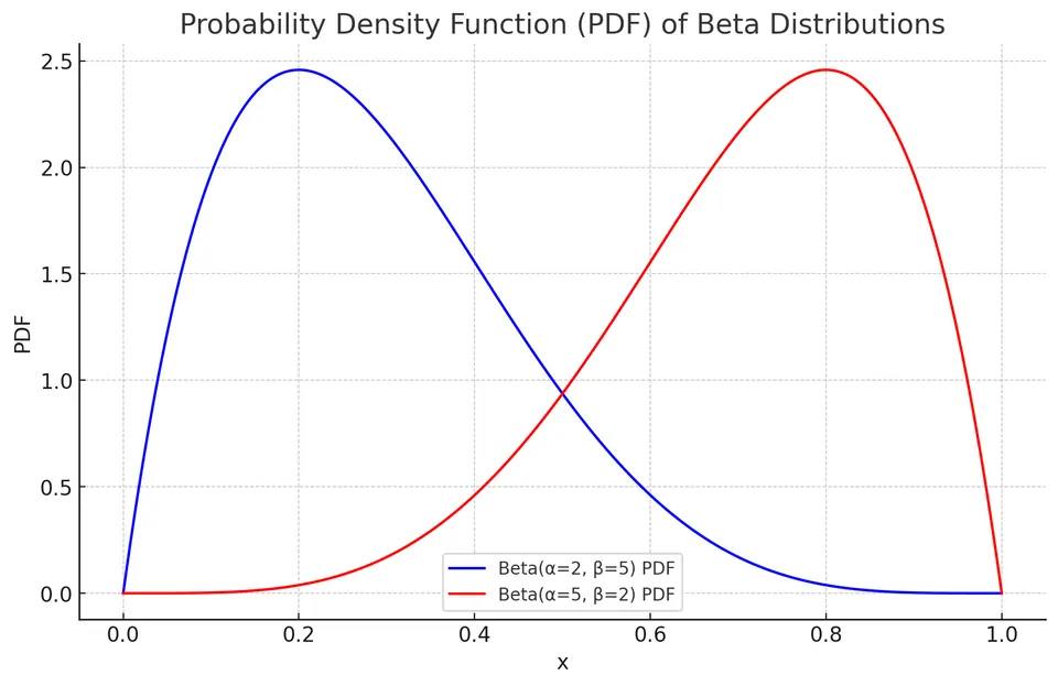
A continuous random variable $X$ follows a beta distribution when its support is the interval $[0,1]$ and its shape is governed by two positive parameters. The beta distribution is denoted as $X \sim \text{Beta}(\alpha, \beta)$, where $\alpha$ and $\beta$ are shape parameters. A shifted and scaled beta distribution can be used for variables constrained to other finite intervals.

Probability Density Function (PDF)

The PDF of a beta distribution is given by:

$$f(x; \alpha, \beta) = \frac{x^{\alpha - 1}(1 - x)^{\beta - 1}}{B(\alpha, \beta)}$$

for $0 \le x \le 1$ and $\alpha, \beta > 0$, where $B(\alpha, \beta)$ is the beta function.

Cumulative Distribution Function (CDF)

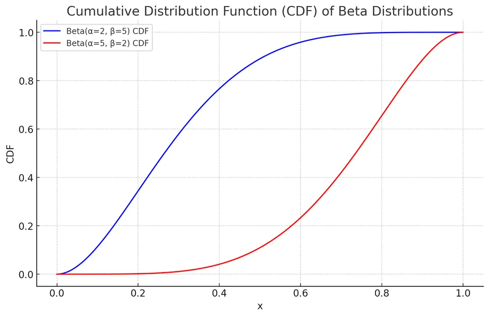
The CDF of a beta distribution, $F(x; \alpha, \beta)$, does not have a simple closed-form expression but is the integral of the PDF over its domain.

Expected Value and Variance

The expected value (mean) of a beta distribution is:

$$E[X] = \frac{\alpha}{\alpha + \beta}$$

The variance of a beta distribution is:

$$\text{Var}(X) = \frac{\alpha \beta}{(\alpha + \beta)^2(\alpha + \beta + 1)}$$

Example: Quality Control in Manufacturing

In a manufacturing process, the proportion of defective items produced is assumed to follow a beta distribution with $\alpha = 2$ and $\beta = 5$.

Given:

• $\alpha = 2$
• $\beta = 5$

Using the beta distribution formulas:

I. What is the expected proportion of defective items?

Expected proportion of defective items:

$$E[X] = \frac{2}{2 + 5} \approx 0.2857$$

II. What is the variance of this proportion?

Variance of the proportion:

$$\text{Var}(X) = \frac{2 \times 5}{(2 + 5)^2(2 + 5 + 1)} \approx 0.0255$$

Applications

Beta distributions are widely used in Bayesian statistics and to model probabilities, proportions, and rates on $[0,1]$. Shifted and scaled beta families are also used in project-management models such as PERT. Other applications include reliability engineering, genetics, and ecology.