Negative Binomial Distribution
The negative binomial distribution extends geometric waiting from the first success to the $r$-th success. Repeat independent Bernoulli trials with a common success probability $p$ and stop when the required positive integer number $r$ of successes has occurred.
Here $X$ counts the total number of trials, including the successful ones. Write $X\sim\mathrm{NegBinomial}(r,p)$, with $X\in\{r,r+1,\ldots\}$ and $0<p<1$. The number of failures before stopping is a different variable, $Y=X-r$, whose support begins at 0. In particular, scipy.stats.nbinom uses that failures convention.
Deriving the probability mass function
For the experiment to stop on trial $k$, the final trial must succeed. Among the first $k-1$ trials there must be exactly $r-1$ successes, which can occupy $\binom{k-1}{r-1}$ sets of positions. Every qualifying sequence contains $r$ successes and $k-r$ failures, so
$$ P(X=k)=\binom{k-1}{r-1}p^r(1-p)^{k-r},\qquad k=r,r+1,\ldots. $$
Using $\binom kr$ would include arrangements that reached the target before trial $k$. Requiring the last success to be at the stopping date is what gives the correct coefficient.
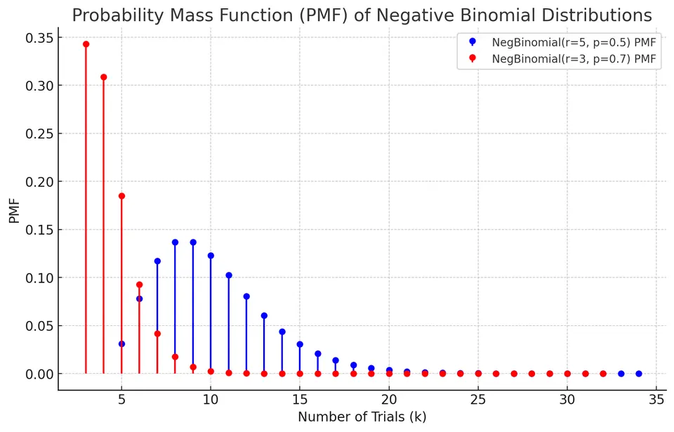
When comparing a plotted count with a formula, check whether the horizontal coordinate counts total trials or failures. A shift by $r$ changes the labels, not the probabilities of the corresponding events.
Cumulative distribution function
For an integer $k\ge r$,
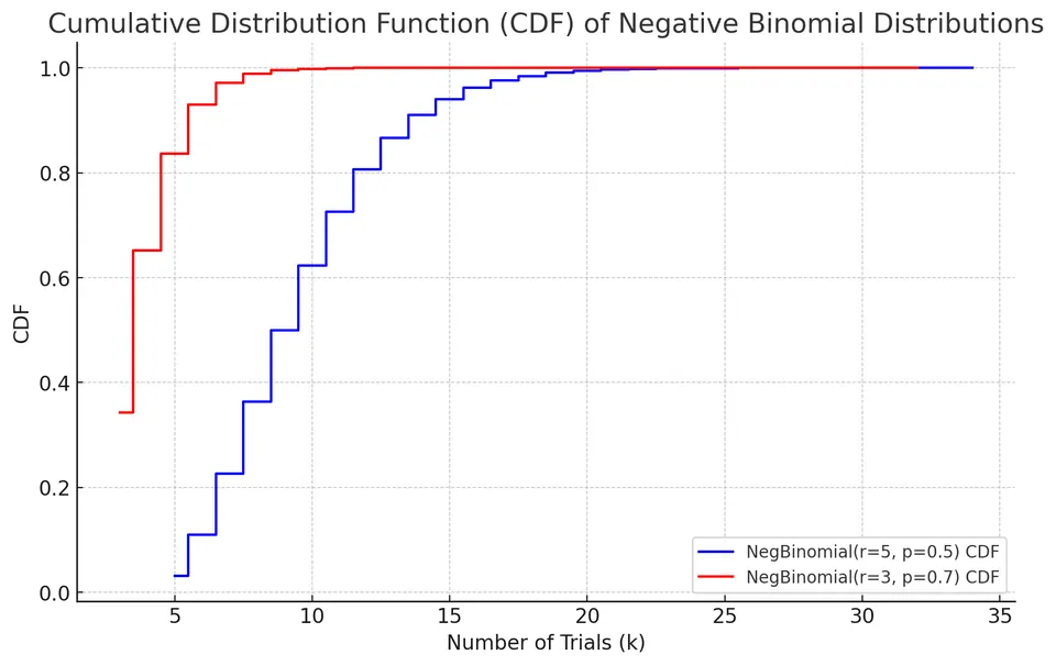
$$ F(k)=P(X\le k)=\sum_{i=r}^{k}\binom{i-1}{r-1}p^r(1-p)^{i-r}. $$
The CDF is zero below $r$; for noninteger thresholds use the integer floor. An equivalent way to describe $X\le k$ is that at least $r$ successes have occurred in the first $k$ Bernoulli trials. Consequently, the same probability can be calculated as a binomial upper tail. The identity connects a stopping-time question to a fixed-trial count question.
Mean, variance, and generating function
Split the total wait into $r$ successive waits for one success. Under the independent, constant-$p$ trial model, these are independent geometric variables. Adding their means and variances gives
$$ E[X]=\frac rp,\qquad \mathrm{Var}(X)=\frac{r(1-p)}{p^2}. $$
Their MGFs multiply as well:
$$ M_X(t)=\left(\frac{pe^t}{1-(1-p)e^t}\right)^r, \qquad t<-\ln(1-p). $$
For $Y=X-r$, the mean becomes $r(1-p)/p$, but the variance is unchanged because subtracting a constant does not change spread. This explains why a software mean can differ from the formula for $X$ without either calculation being wrong. If $p=1$, exactly $r$ trials are needed and the variance is zero.
Example: quality-control testing
An inspector tests independent products until finding five defective items. Label “defective” a success, take $p=0.1$, and let $r=5$. Calling a defect a success is only a counting convention; it does not change its practical meaning.
Exactly 20 products tested
The first 19 products must contain four defects, and product 20 must be defective:
$$ P(X=20)=\binom{19}{4}(0.1)^5(0.9)^{15}\approx0.0080. $$
Under the failures convention this same event is $Y=15$, so a software calculation uses the failure count 15, not the total count 20.
Expected number of products
$$ E[X]=\frac5{0.1}=50. $$
Five separate mean waits of 10 trials add to an expected total of 50.
Variance of the total
$$ \mathrm{Var}(X)=\frac{5(1-0.1)}{0.1^2}=450. $$
The standard deviation is $\sqrt{450}\approx21.21$ trials. The failures variable has mean 45 and the same variance 450.
Applications and conventions
This waiting-time construction applies to inspection, repeated reliability attempts, and other experiments that stop after a specified count of the event of interest. Negative binomial models are also used for variable count data in epidemiology and ecology, but a count-regression parameterization need not literally describe waiting for an integer number of successes. Identify the support, the counted quantity, and the parameter definitions before transferring formulas between uses.
Practice: Exercises with worked solutions